Section 8.1 Weighing Penguins
Suppose you are a researcher in Antarctica, studying local populations of penguins. One of your tasks is to monitor the average weight of the penguins as it varies over the course of the year. It would be impractical to weigh every penguin in the environment, so your plan is to collect a random sample of 10 penguins each week, weigh them, and use the sample to estimate the mean of the entire population -- which is called the population mean.
There are many ways you could use the sample to estimate the population mean, but we’ll consider just two: the sample mean and the sample median. They are both reasonable choices, but let’s see which is better -- and think about what we mean by "better".
For purposes of demonstration, we’ll assume that penguin weights are drawn from a normal distribution with known mean and standard deviation, which I’ll denote
mu and sigma and assign values in kilograms.
mu = 3.7
sigma = 0.46
These values are the parameters of the normal distribution, which means that they specify a particular distribution. Given these parameters, we can use NumPy to simulate the sampling process and generate a sample of any size. For example, here’s a hypothetical sample of 10 weights.
# Seed the random number generator so we get the same results every time
np.random.seed(1)
$ sample = np.random.normal(mu, sigma, size=10)
sample
array([4.44719887, 3.41859205, 3.45704099, 3.20643443, 4.09808751,
       2.6412922 , 4.50261341, 3.34984483, 3.84675798, 3.58528963])
And here are the mean and median of the sample.
$ np.mean(sample), np.median(sample)
(np.float64(3.6553151902291945), np.float64(3.521165310619601))
The mean and median are different enough that we should wonder which is a better estimate. To find out, we’ll use the following function to generate hypothetical samples with the given size,
n.
def make_sample(n):
    return np.random.normal(mu, sigma, size=n)
As a first experiment, let’s see how the sample mean and sample median behave as the sample size increases. We’ll use the NumPy function
logspace to make a range of ns from 10 to 100,000, equally spaced on a logarithmic scale.
ns = np.logspace(1, 5).astype(int)
We can use a list comprehension to generate a hypothetical sample for each value of
n, compute the mean, and collect the results:
means = [np.mean(make_sample(n)) for n in ns]
And we’ll do the same for the median.
medians = [np.median(make_sample(n)) for n in ns]
A statistic, like the sample mean or median, that’s used to estimate a property of a population is called an estimator.
The following figure shows how these estimators behave as we increase the sample size. The horizontal line shows the actual mean in the population.
plt.axhline(mu, color="gray", lw=1, alpha=0.5)
plt.plot(ns, means, "--", label="mean")
plt.plot(ns, medians, alpha=0.5, label="median")

decorate(xlabel="Sample size", xscale="log", ylabel="Estimate")
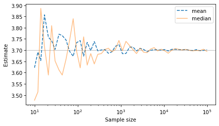
For both estimators, the estimates converge to the actual value as the sample size increases. This demonstrates that they are consistent, which is one of the properties a good estimator should have. Based on this property, the mean and median seem equally good.
In the previous figure, you might notice that the estimates are sometimes too high and sometimes too low -- and it looks like the variation is roughly symmetric around the true value. That suggests another experiment: if we collect many samples with the same size and compute many estimates, what is the average of the estimates?
The following loop simulates this scenario by generating 10,001 samples of 10 penguins and computing the mean of each sample.
$ means = [np.mean(make_sample(n=10)) for i in range(10001)]
np.mean(means)
np.float64(3.7003450849286907)
The average of the means is close to the actual mean we used to generate the samples: 3.7 kg.
The following loop simulates the same scenario, but this time it computes the median of each sample.
$ medians = [np.median(make_sample(n=10)) for i in range(10001)]
np.mean(medians)
np.float64(3.701214089907223)
The average of these hypothetical medians is also very close to the actual population mean.
These results demonstrate that the sample mean and median are unbiased estimators, which means that they are correct on average. The word "bias" means different things in different contexts, which can be a source of confusion. In this context, "unbiased" means that the average of the estimates is the actual value.
So far, we’ve shown that both estimators are consistent and unbiased, but it’s still not clear which is better. Let’s try one more experiment: let’s see which estimator is more accurate. The word "accurate" also means different things in different contexts -- as one way to quantify it, let’s consider the mean squared error (MSE). The following function computes the differences between the estimates and the actual value, and returns the mean of the squares of these errors.
def mse(estimates, actual):
    """Mean squared error of a sequence of estimates."""
    errors = np.asarray(estimates) - actual
    return np.mean(errors**2)
Notice that we can only compute MSE if we know the actual value. In practice, we usually don’t -- after all, if we knew the actual value, we wouldn’t have to estimate it. But in our experiment, we know that the actual population mean is 3.7 kg, so we can use it to compute the MSE of the sample means.
$ mse(means, mu)
np.float64(0.020871984891289382)
If we have samples with size 10 and we use the sample mean to estimate the population mean, the average squared error is about 0.021 kilograms squared. Now here’s the MSE of the sample medians.
$ mse(medians, mu)
np.float64(0.029022273128644173)
If we use the sample medians to estimate the population mean, the average squared error is about 0.029 kilograms squared. In this example, the sample mean is better than the sample median; and in general, if the data are drawn from a normal distribution, it is the best unbiased estimator of the population mean, in the sense that it minimizes MSE.
Minimizing MSE is a good property for an estimator to have, but MSE is not always the best way to summarize errors. For one thing, it is hard to interpret. In this example, the units of MSE are kilograms squared, so it’s hard to say what that means.
One solution is to use the square root of MSE, called "root mean squared error", or RMSE. Another option is to use the average of the absolute values of the errors, called the "mean absolute error" or MAE. The following function computes MAE for a sequence of estimates.
def mae(estimates, actual):
    """Mean absolute error of a sequence of estimates."""
    errors = np.asarray(estimates) - actual
    return np.mean(np.abs(errors))
Here’s the MAE of the sample means.
$ mae(means, mu)
np.float64(0.1154043374950527)
And the sample medians.
$ mae(medians, mu)
np.float64(0.13654429774596036)
On average, we expect the sample mean to be off by about 0.115 kg, and the sample median to be off by 0.137 kg. So the sample mean is probably the better choice, at least for this example.

