Prediction with ARIMA

Section 12.9 Prediction with ARIMA

The object returned by ARIMA provides a method called get_forecast that generates predictions. To demonstrate, we’ll split the time series into a training and test set, and fit the same model to the training set.

🔗

Listing 12.9.1. Python Code

🔗

training, test = split_series(nuclear)
model = tsa.ARIMA(training, order=order, seasonal_order=seasonal_order)
results_training = model.fit()

We can use the result to generate a forecast for the test set.

🔗

Listing 12.9.2. Python Code

🔗

forecast = results_training.get_forecast(steps=len(test))

The result is an object that contains an attribute called forecast_mean and a function that returns a confidence interval.

🔗

Listing 12.9.3. Python Code

🔗

forecast_mean = forecast.predicted_mean
forecast_ci = forecast.conf_int()
forecast_ci.columns = ["lower", "upper"]

We can plot the results like this and compare them to the actual time series.

🔗

Listing 12.9.4. Python Code

🔗

plt.fill_between(
    forecast_ci.index,
    forecast_ci.lower,
    forecast_ci.upper,
    lw=0,
    color="gray",
    alpha=0.2,
)
plt.plot(forecast_mean.index, forecast_mean, label="forecast", **pred_options)
plt.plot(test.index, test, label="actual", **actual_options)
decorate(ylabel="GWh")

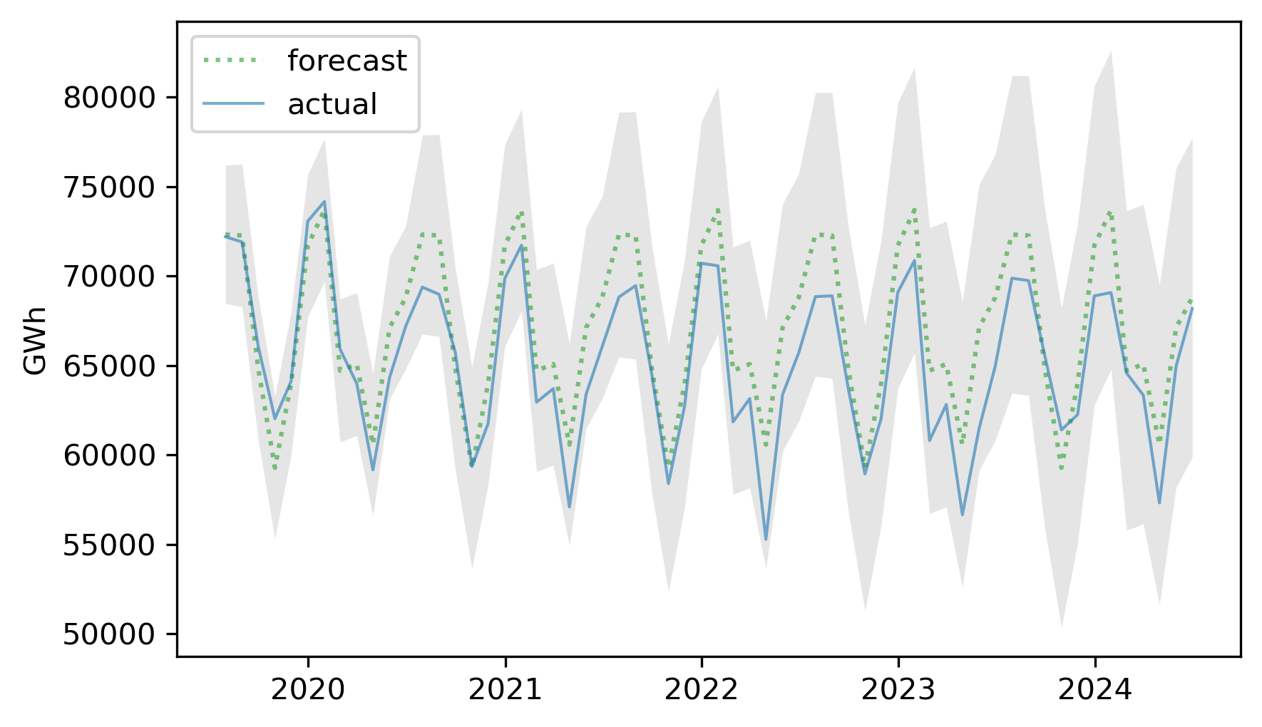
The actual values fall almost entirely within the confidence interval of the predictions. Here’s the MAPE of the predictions.

🔗

Listing 12.9.6. Python Code

🔗

$ MAPE(forecast_mean, test)
np.float64(3.3817549248044547)

The predictions are off by 3.38% on average, somewhat better than the results we got from seasonal decomposition (3.81%).

🔗

ARIMA is more versatile than seasonal decomposition, and can often make better predictions. In this time series, the autocorrelations are not especially strong, so the advantage of ARIMA is modest.

🔗

Prev Top Next