Least Squares Fit

Section 10.1 Least Squares Fit

As a first example, let’s return to the scenario from Chapter 8. Suppose you are a researcher in Antarctica, studying local populations of penguins. As part of your data collection, you capture a sample of penguins, measure and weigh them -- and then release them unharmed.

🔗

As you would soon learn, it can be difficult to get penguins to stay on the scale long enough to get an accurate measurement. Suppose that for some penguins we have measurements like flipper and bill sizes, but no weights. Let’s see if we can use the other measurements to fill in the missing data -- this process is called imputation.

🔗

We’ll start by exploring the relationship between the weights and measurements, using data collected between 2007 and 2010 by researchers at Palmer Station in Antarctica. The data they collected is freely available -- instructions for downloading it are in the notebook for this chapter.

🔗

The following cell downloads the data from a repository created by Allison Horst.

🔗

Horst AM, Hill AP, Gorman KB (2020). palmerpenguins: Palmer Archipelago (Antarctica) penguin data. R package version 0.1.0. https://allisonhorst.github.io/palmerpenguins/. doi: 10.5281/zenodo.3960218.

🔗

The data was collected as part of the research that led to this paper: Gorman KB, Williams TD, Fraser WR (2014). Ecological sexual dimorphism and environmental variability within a community of Antarctic penguins (genus Pygoscelis). PLoS ONE 9(3):e90081. https://doi.org/10.1371/journal.pone.0090081

🔗

Listing 10.1.1. Python Code

🔗

download(
    "https://raw.githubusercontent.com/allisonhorst/palmerpenguins/c19a904462482430170bfe2c718775ddb7dbb885/inst/extdata/penguins_raw.csv"
)

We can use read_csv to read the data.

🔗

Listing 10.1.2. Python Code

🔗

$ penguins = pd.read_csv("penguins_raw.csv").dropna(subset=["Body Mass (g)"])
penguins.shape
(342, 17)

The dataset includes measurements of 151 Adélie penguins. We can use query to select the rows that contain this data.

🔗

Listing 10.1.3. Python Code

🔗

$ adelie = penguins.query('Species.str.startswith("Adelie")')
len(adelie)
151

Now suppose we know the flipper length of an Adélie penguin -- let’s see how well we can predict its weight. First we’ll select these columns from the DataFrame.

🔗

Listing 10.1.4. Python Code

🔗

xvar = "Flipper Length (mm)"
yvar = "Body Mass (g)"

flipper_length = adelie[xvar]
body_mass = adelie[yvar]

Here’s a scatter plot showing the relationship between these quantities.

🔗

Listing 10.1.5. Python Code

🔗

plt.scatter(flipper_length, body_mass, marker=".", alpha=0.5)
decorate(xlabel=xvar, ylabel=yvar)

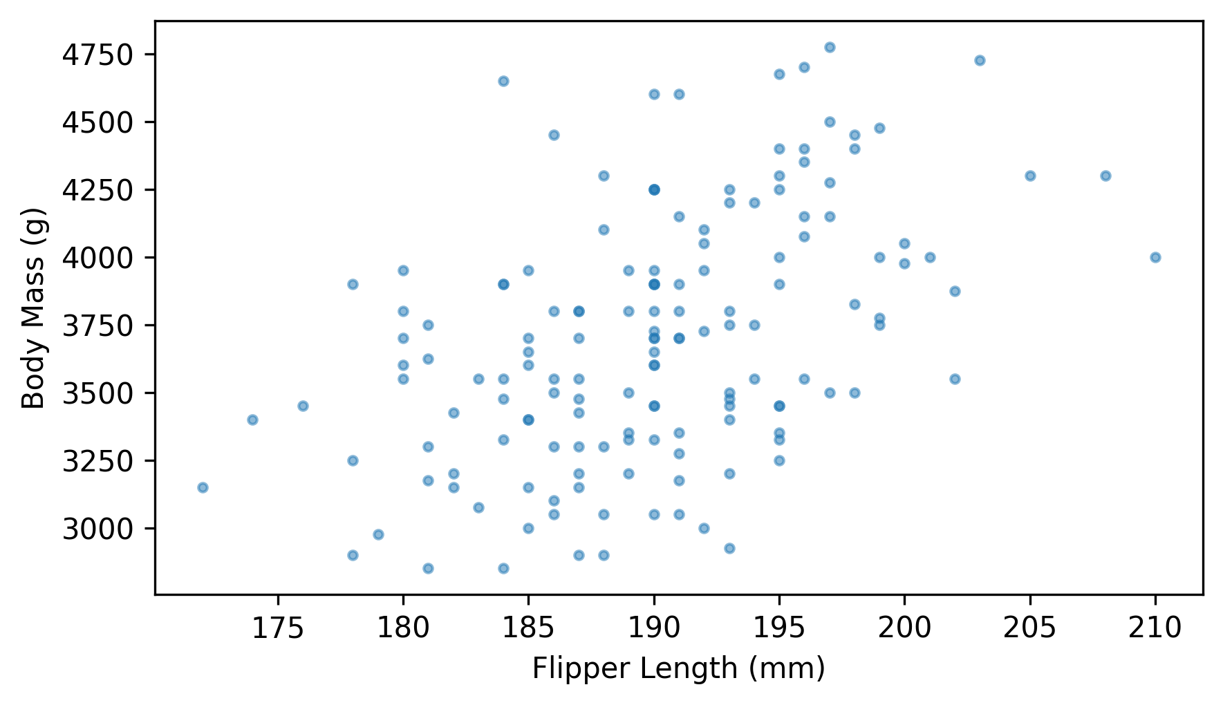
It looks like they are related -- we can quantify the strength of the relationship by computing the coefficient of correlation.

🔗

Listing 10.1.7. Python Code

🔗

$ np.corrcoef(flipper_length, body_mass)[0, 1]
np.float64(0.4682016942179394)

The correlation is about 0.47, so penguins with longer flippers tend to be heavier. That’s useful because it means we can guess a penguin’s weight more accurately if we know its flipper length -- but correlation alone doesn’t tell us how to make those guesses. For that, we need to choose a line of best fit.

🔗

There are many ways to define the "best" line, but for data like this a common choice is a linear least squares fit, which is the straight line that minimizes the mean squared error (MSE).

🔗

SciPy provides a function called linregress that computes a least squares fit. The name is short for linear regression, which is another term for a model like this. The arguments of linregress are the x values and the y values, in that order.

🔗

Listing 10.1.8. Python Code

🔗

$ from scipy.stats import linregress

result = linregress(flipper_length, body_mass)
result
LinregressResult(slope=np.float64(32.83168975115009), intercept=np.float64(-2535.8368022002514), rvalue=np.float64(0.46820169421793933), pvalue=np.float64(1.3432645947790051e-09), stderr=np.float64(5.076138407990821), intercept_stderr=np.float64(964.7984274994059))

The result is a LinregressResult object that contains the slope and intercept of the fitted line, along with other information we’ll unpack soon. The slope is about 32.8, which means that each additional millimeter of flipper length is associated with an additional 32.8 grams of body weight.

🔗

The intercept is -2535 grams, which might seem nonsensical, since a measured weight can’t be negative. It might make more sense if we use the slope and intercept to evaluate the fitted line at the average flipper length.

🔗

Listing 10.1.9. Python Code

🔗

$ x = flipper_length.mean()
y = result.intercept + result.slope * x
x, y
(np.float64(189.95364238410596), np.float64(3700.662251655629))

For a penguin with the average flipper length, about 190 mm, the expected body weight is about 3700 grams.

🔗

The following function takes the result from linregress and a sequence of xs and finds the point on the fitted line for each value of x.

🔗

Listing 10.1.10. Python Code

🔗

def predict(result, xs):
    ys = result.intercept + result.slope * xs
    return ys

The name predict might seem odd here -- in natural language, a prediction usually pertains to something happening in the future, but in the context of regression, the points on the fitted line are also called predictions.

🔗

We can use predict to compute the points on the line for a range of flipper sizes.

🔗

Listing 10.1.11. Python Code

🔗

fit_xs = np.linspace(np.min(flipper_length), np.max(flipper_length))
fit_ys = predict(result, fit_xs)

Here’s the fitted line along with the scatter plot of the data.

🔗

Listing 10.1.12. Python Code

🔗

plt.scatter(flipper_length, body_mass, marker=".", alpha=0.5)
plt.plot(fit_xs, fit_ys, color="C1")
decorate(xlabel=xvar, ylabel=yvar)

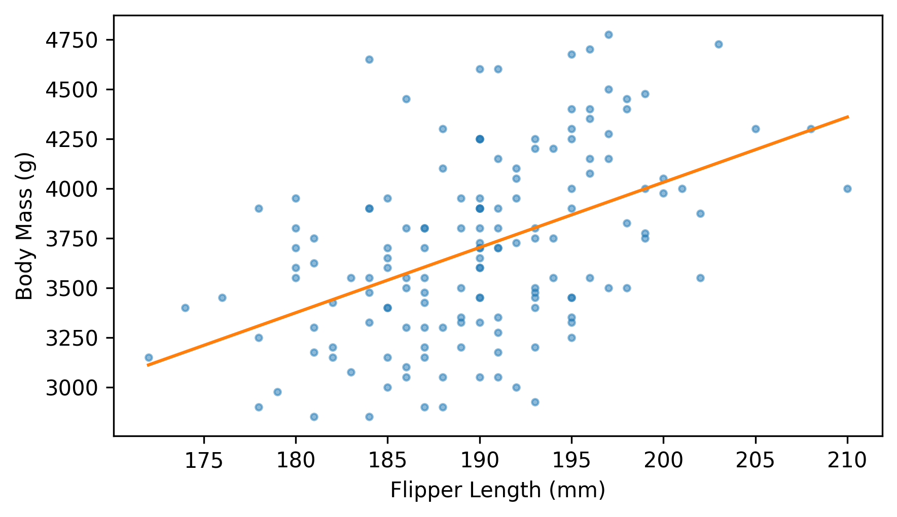
As expected, the fitted line goes through the center of the data and follows the trend. And some of the predictions are accurate -- but many of the data points are far from the line. To get a sense of how good (or bad) the predictions are, we can compute the prediction error, which is the vertical distance of each point from the line. The following function computes these errors, which are also called residuals.

🔗

Listing 10.1.14. Python Code

🔗

def compute_residuals(result, xs, ys):
    fit_ys = predict(result, xs)
    return ys - fit_ys

Here are the residuals for body mass as a function of flipper length.

🔗

Listing 10.1.15. Python Code

🔗

residuals = compute_residuals(result, flipper_length, body_mass)

As an example, we can look at the results for the first penguin in the dataset.

🔗

Listing 10.1.16. Python Code

🔗

$ x = flipper_length[0]
y = predict(result, x)
x, y
(np.float64(181.0), np.float64(3406.699042757914))

The flipper length of the selected penguin is 181 mm and the predicted body mass is 3407 grams. Now let’s see what the actual mass is.

🔗

Listing 10.1.17. Python Code

🔗

$ body_mass[0], residuals[0]
(np.float64(3750.0), np.float64(343.30095724208604))

The actual mass of this penguin is 3750 grams, and the residual -- after subtracting away the prediction -- is 343 grams.

🔗

The average of the squared residuals is the mean squared error (MSE) of the predictions.

🔗

Listing 10.1.18. Python Code

🔗

$ mse = np.mean(residuals**2)
mse
np.float64(163098.85902884745)

By itself, this number doesn’t mean very much. We can make more sense of it by computing the coefficient of determination.

🔗

Prev Top Next