Retrodiction with Autoregression

Section 12.7 Retrodiction with Autoregression

To generate retrodictions, we’ll start by putting the year-over-year differences in a Series that’s aligned with the index of the original.

🔗

Listing 12.7.1. Python Code

🔗

pred_diff = pd.Series(pred_diff, index=nuclear.index)

Using isna to check for NaN values, we find that the first 21 elements of the new Series are missing.

🔗

Listing 12.7.2. Python Code

🔗

$ n_missing = pred_diff.isna().sum()
n_missing
np.int64(21)

That’s because we shifted the Series by 12 months to compute year-over-year differences, then we shifted the differences 3 months for the first autoregression model, and we shifted the residuals of the first model by 6 months for the second model. Each time we shift a Series like this, we lose a few values at the beginning, and the sum of these shifts is 21.

🔗

So before we can generate retrodictions, we have to prime the pump by copying the first 21 elements from the original into a new Series.

🔗

Listing 12.7.3. Python Code

🔗

pred_series = pd.Series(index=nuclear.index, dtype=float)
pred_series.iloc[:n_missing] = nuclear.iloc[:n_missing]

Now we can run the following loop, which fills in the elements from index 21 (which is the 22nd element) to the end. Each element is the sum of the value from the previous year and the predicted year-over-year difference.

🔗

Listing 12.7.4. Python Code

🔗

for i in range(n_missing, len(pred_series)):
    pred_series.iloc[i] = pred_series.iloc[i - 12] + pred_diff.iloc[i]

Now we’ll replace the elements we copied with NaN so we don’t get credit for "predicting" the first 21 values perfectly.

🔗

Listing 12.7.5. Python Code

🔗

pred_series[:n_missing] = np.nan

Here’s what the retrodictions look like compared to the original.

🔗

Listing 12.7.6. Python Code

🔗

pred_series.plot(label="predicted", **pred_options)
nuclear.plot(label="actual", **actual_options)
decorate(ylabel="GWh")

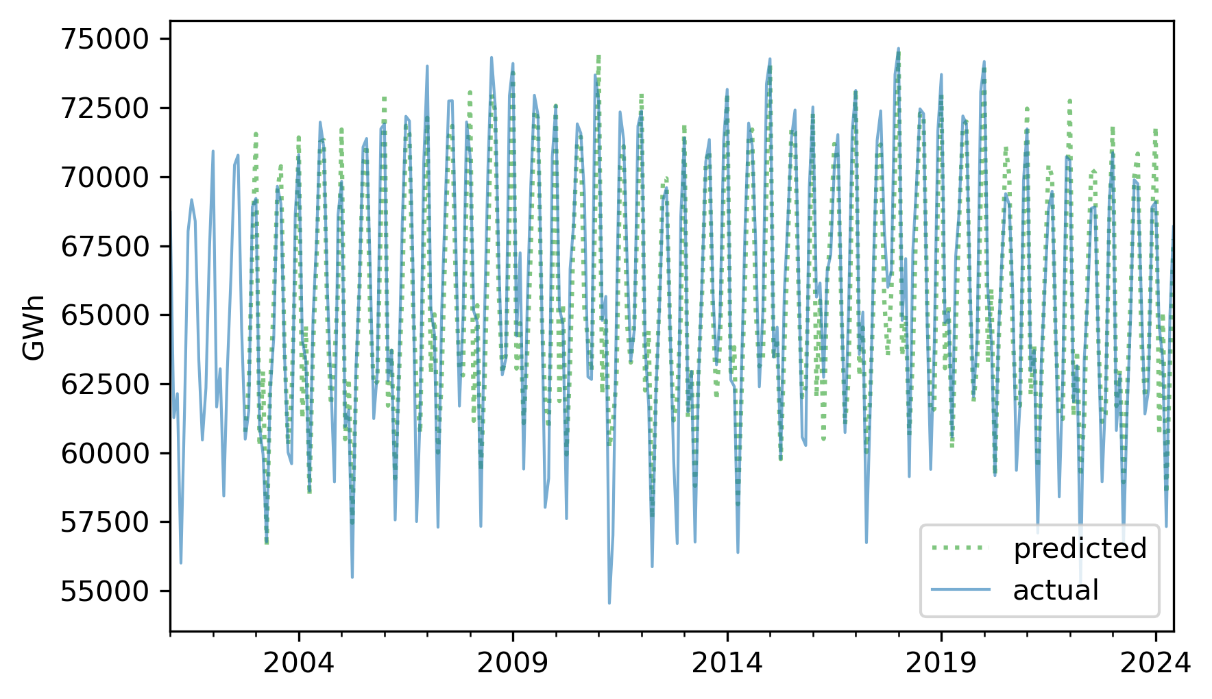
They look pretty good, and the \(R^2\) value is about 0.86.

🔗

Listing 12.7.8. Python Code

🔗

$ resid = (nuclear - pred_series).dropna()
R2 = 1 - resid.var() / nuclear.var()
R2
np.float64(0.8586566911201015)

The model we used to compute these retrodictions is called SARIMA, which is one of a family of models called ARIMA. Each part of these acronyms refers to an element of the model.

🔗

S stands for seasonal, because the first step was to compute differences between values separated by one seasonal period.
🔗

🔗
AR stands for autoregression, which we used to model lagged correlations in the differences.
🔗

🔗
I stands for integrated, because the iterative process we used to compute pred_series is analogous to integration in calculus.
🔗

🔗
MA stands for moving average, which is the conventional name for the second autoregression model we ran with the residuals from the first.
🔗

🔗

ARIMA models are powerful and versatile tools for modeling time series data.

🔗

Prev Top Next