Marriage Data

Section 13.3 Marriage Data

In many countries, people are getting married later than they used to, and more people stay unmarried. To explore these trends in the United States, we’ll use the tools of survival analysis and data from the National Survey of Family Growth (NSFG).

🔗

The NSFG dataset we used in previous chapters is the pregnancy file, which contains one row for each pregnancy reported by the survey respondents. In this chapter, we’ll work with the respondent file, which contains information about the respondents themselves.

🔗

I have compiled responses from nine iterations of the survey, conducted between 1982 and 2019, and selected data related to marriage.

🔗

The following cell downloads the data, which is a CSV file I created that combines data from several iterations of the NSFG survey, from 1982 to 2019. Details of the data preparation are in this notebook.

🔗

Listing 13.3.1. Python Code

🔗

filename = "marriage_nsfg_female.csv.gz"
download("https://github.com/AllenDowney/ThinkStats/raw/v3/data/" + filename)

We can read the data like this.

🔗

Listing 13.3.2. Python Code

🔗

resp = pd.read_csv("marriage_nsfg_female.csv.gz")
resp.shape

(70183, 34)

The excerpt includes one row for each of more than 70,000 respondents, and has the following variables related to age and marriage.

🔗

cmbirth: The respondent’s date of birth, known for all respondents.
🔗

🔗
cmintvw: The date the respondent was interviewed, known for all respondents.
🔗

🔗
cmmarrhx: The date the respondent was first married, if applicable and known.
🔗

🔗
evrmarry: 1 if the respondent had been married prior to the date of interview, 0 otherwise.
🔗

🔗

The first three variables are encoded in “century-months”—that is, the integer number of months since December 1899. So century-month 1 is January 1900.

🔗

To explore generational changes, we’ll group respondents by their decade of birth. We’ll use the following function, which takes a value of cmbirth and computes the corresponding decade of birth. It uses the integer division operator // to divide by 10 and round down.

🔗

Listing 13.3.3. Python Code

🔗

month0 = pd.to_datetime("1899-12-31")


def decade_of_birth(cmbirth):
    date = month0 + pd.DateOffset(months=cmbirth)
    return date.year // 10 * 10

We can use this function and the apply method to compute each respondent’s decade of birth and assign it to a new column called cohort. In this context, a cohort is a group of people with something in common—like the decade they were born—who are treated as a group for purposes of analysis.

🔗

The result from value_counts shows the number of people in each cohort.

🔗

Listing 13.3.4. Python Code

🔗

from thinkstats import value_counts

resp["cohort"] = resp["cmbirth"].apply(decade_of_birth)
value_counts(resp["cohort"])

cohort
1930      325
1940     3608
1950    10631
1960    14953
1970    16438
1980    14271
1990     8552
2000     1405
Name: count, dtype: int64

The dataset includes more than 10,000 respondents born in each decade from the 1950s to the 1980s, and fewer respondents in the earlier and later decades.

🔗

Next we’ll compute each respondent’s age when married (if applicable) and their age when interviewed.

🔗

Listing 13.3.5. Python Code

🔗

resp["agemarr"] = (resp["cmmarrhx"] - resp["cmbirth"]) / 12
resp["age"] = (resp["cmintvw"] - resp["cmbirth"]) / 12

To get started with this data, we’ll use the following function, which takes as arguments a DataFrame and a list of cohorts, and returns a dictionary that maps from each cohort to a Surv object. For each cohort, it selects their ages at first marriage and uses Surv.from_seq to compute a survival function. The dropna=False argument includes NaN values in the survival function, so the result includes people who have not married.

🔗

Listing 13.3.6. Python Code

🔗

from empiricaldist import Surv


def make_survival_map(resp, cohorts):
    surv_map = {}

    grouped = resp.groupby("cohort")
    for cohort in cohorts:
        group = grouped.get_group(cohort)
        surv_map[cohort] = Surv.from_seq(group["agemarr"], dropna=False)

    return surv_map

Here’s how we use this function.

🔗

Listing 13.3.7. Python Code

🔗

cohorts = [1980, 1960, 1940]
surv_map = make_survival_map(resp, cohorts)

And here are the results for people born in the 1940s, 1960s, and 1980s.

🔗

Listing 13.3.8. Python Code

🔗

import matplotlib.pyplot as plt
import cycler

# Extract the default color cycle
default_colors = plt.rcParams["axes.prop_cycle"].by_key()["color"]

# Define the desired line styles
linestyles = ["--", "-", "-.", "--", "-", "-.", "--", "-", "-.", "--"]

# Ensure we cycle through styles and colors properly
custom_cycler = cycler.cycler(color=default_colors) + cycler.cycler(
    linestyle=linestyles
)

# Apply the new cycler
plt.rc("axes", prop_cycle=custom_cycler)

Listing 13.3.9. Python Code

🔗

for cohort, surv in surv_map.items():
    surv.plot(label=f"{cohort}s")

ylim = [-0.05, 1.05]
decorate(xlabel="Age", ylabel="Prob never married", ylim=ylim)

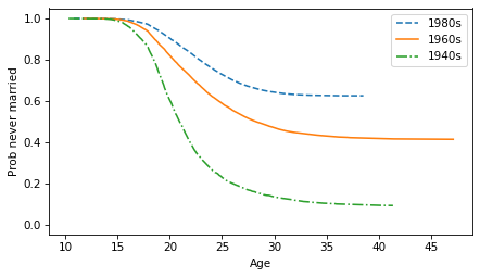
If we take these results at face value, they show that people in earlier generations got married younger, and more of them got married eventually. However, we should not interpret these results yet, because they are not correct. There are two problems we have to address:

🔗

As discussed in Chapter 1, the NSFG uses stratified sampling, which means that it deliberately oversamples some groups.
🔗

🔗
Also, this way of computing the survival function does not properly take into account people who are not married yet.
🔗

🔗

For the first problem, we’ll use a kind of resampling called a weighted bootstrap. For the second problem, we’ll use a method called Kaplan-Meier estimation. We’ll start with resampling.

🔗

Prev Top Next