Section 6.2 Probability Density
We’ll start with the probability density function (PDF) of the normal distribution, which computes the density for the quantities,
xs, given mu and sigma.
def normal_pdf(xs, mu, sigma):
    """Evaluates the normal probability density function."""
    z = (xs - mu) / sigma
    return np.exp(-(z**2) / 2) / sigma / np.sqrt(2 * np.pi)
m, s = np.mean(trimmed), np.std(trimmed)
Now we’ll evaluate
normal_pdf for a range of weights.
low = m - 4 * s
high = m + 4 * s
qs = np.linspace(low, high, 201)
ps = normal_pdf(qs, m, s)
And plot it.
plt.plot(qs, ps, label="normal model", ls=":", color="gray")
decorate(xlabel="Birth weight (pounds)", ylabel="Density")
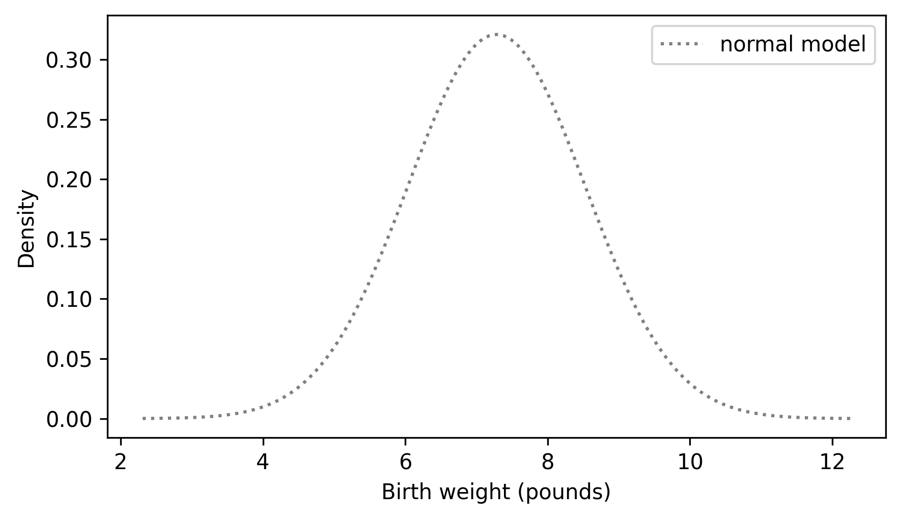
The result looks like a bell curve, which is characteristic of the normal distribution.
When we evaluate
normal_pdf, the result is a probability density. For example, here’s the density function evaluated at the mean, which is where the density is highest.
$ normal_pdf(m, m, s)
np.float64(0.32093416297880123)
By itself, a probability density doesn’t mean much — most importantly, it is not a probability. It would be incorrect to say that the probability is 32% that a randomly-chosen birth weight equals
m. In fact, the probability that a birth weight is truly, exactly, and precisely equal to m — or any other specific value — is zero.
However, we can use the probability densities to compute the probability that an outcome falls in an interval between two values, by computing the area under the curve.
We could do that with the
normal_pdf function, but it is more convenient to use the NormalPdf class, which is defined in the thinkstats module. Here’s how we create a NormalPdf object with the same mean and standard deviation as the birth weights in the NSFG dataset.
$ from thinkstats import NormalPdf

pdf_model = NormalPdf(m, s, name="normal model")
pdf_model
NormalPdf(7.280883100022579, 1.2430657948614345, name='normal model')
If we call this object like a function, it evaluates the normal PDF.
$ pdf_model(m)
np.float64(0.32093416297880123)
Now, to compute the area under the PDF, we can use the following function, which takes a
NormalPdf object and the bounds of an interval, low and high. It evaluates the normal PDF at equally-spaced quantities between low and high, and uses the SciPy function simpson to estimate the area under the curve (simpson is so named because it uses an algorithm called Simpson’s method).
from scipy.integrate import simpson


def area_under(pdf, low, high):
    qs = np.linspace(low, high, 501)
    ps = pdf(qs)
    return simpson(y=ps, x=qs)
If we compute the area under the curve from the lowest to the highest point in the graph, the result is close to 1.
$ area_under(pdf_model, 2, 12)
np.float64(0.9999158086616793)
If we extend the interval from negative infinity to positive infinity, the total area is exactly 1.
If we start from 0 — or any value far below the mean — we can compute the fraction of birth weights less than or equal to 8.5 pounds.
$ area_under(pdf_model, 0, 8.5)
np.float64(0.8366380335513807)
You might recall that the "fraction less than or equal to a given value" is the definition of the CDF. So we could compute the same result using the CDF of the normal distribution.
$ from scipy.stats import norm

norm.cdf(8.5, m, s)
np.float64(0.8366380358092718)
Similarly, we can use the area under the density curve to compute the fraction of birth weights between 6 and 8 pounds.
$ area_under(pdf_model, 6, 8)
np.float64(0.5671317752927691)
Or we can get the same result using the CDF to compute the fraction less than 8 and then subtracting off the fraction less than 6.
$ norm.cdf(8, m, s) - norm.cdf(6, m, s)
np.float64(0.5671317752921801)
So the CDF is the area under the curve of the PDF. If you know calculus, another way to say the same thing is that the CDF is the integral of the PDF. And conversely, the PDF is the derivative of the CDF.

