Section 4.2 CDFs
A cumulative distribution function, or CDF, is another way to describe the distribution of a set of values, along with a frequency table or PMF. Given a value
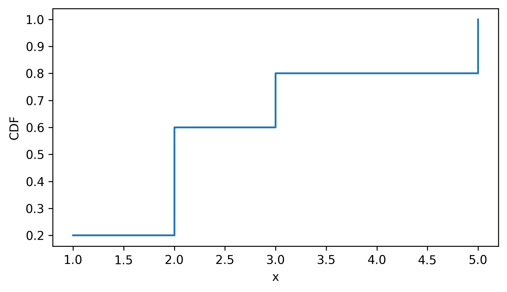
x, the CDF computes the fraction of values less than or equal to x. As an example, we’ll start with a short sequence.
t = [1, 2, 2, 3, 5]
One way to compute a CDF is to start with a PMF. Here is a
Pmf object that represents the distribution of values in t.
$ from empiricaldist import Pmf

pmf = Pmf.from_seq(t)
pmf
1    0.2
2    0.4
3    0.2
5    0.2
Name: , dtype: float64
As we saw in the previous chapter, we can use the bracket operator to look up a value in a
Pmf.
$ pmf[2]
np.float64(0.4)
The result is the proportion of values in the sequence equal to the given value. In this example, two out of five values are equal to
2, so the result is 0.4. We can also think of this proportion as the probability that a randomly chosen value from the sequence equals 2.
$ cdf = pmf.make_cdf()
cdf
1    0.2
2    0.6
3    0.8
5    1.0
Name: , dtype: float64
The result is a
Cdf object, which is a kind of Pandas Series. We can use the bracket operator to look up a value.
$ cdf[2]
np.float64(0.6000000000000001)
The result is the proportion of values in the sequence less than or equal to the given value. In this example, three out of five values in the sequence are less than or equal to
2, so the result is 0.6. We can also think of this proportion as the probability that a randomly chosen value from the sequence is less than or equal to 2.
We can use parentheses to call the
Cdf object like a function.
$ cdf(3)
array(0.8)
The cumulative distribution function is defined for all numbers, not just the ones that appear in the sequence.
$ cdf(4)
array(0.8)
cdf.step()
decorate(xlabel="x", ylabel="CDF")
As a second example, let’s make a
Cdf that represents the distribution of running speeds from the previous section. The Cdf class provides a from_seq function we can use to create a Cdf object from a sequence.
from empiricaldist import Cdf

cdf_speeds = Cdf.from_seq(speeds)
And here’s what it looks like — the vertical line is at my speed.
cdf_speeds.step()
plt.axvline(my_speed, ls=":", color="gray")
decorate(xlabel="Speed (mph)", ylabel="CDF")
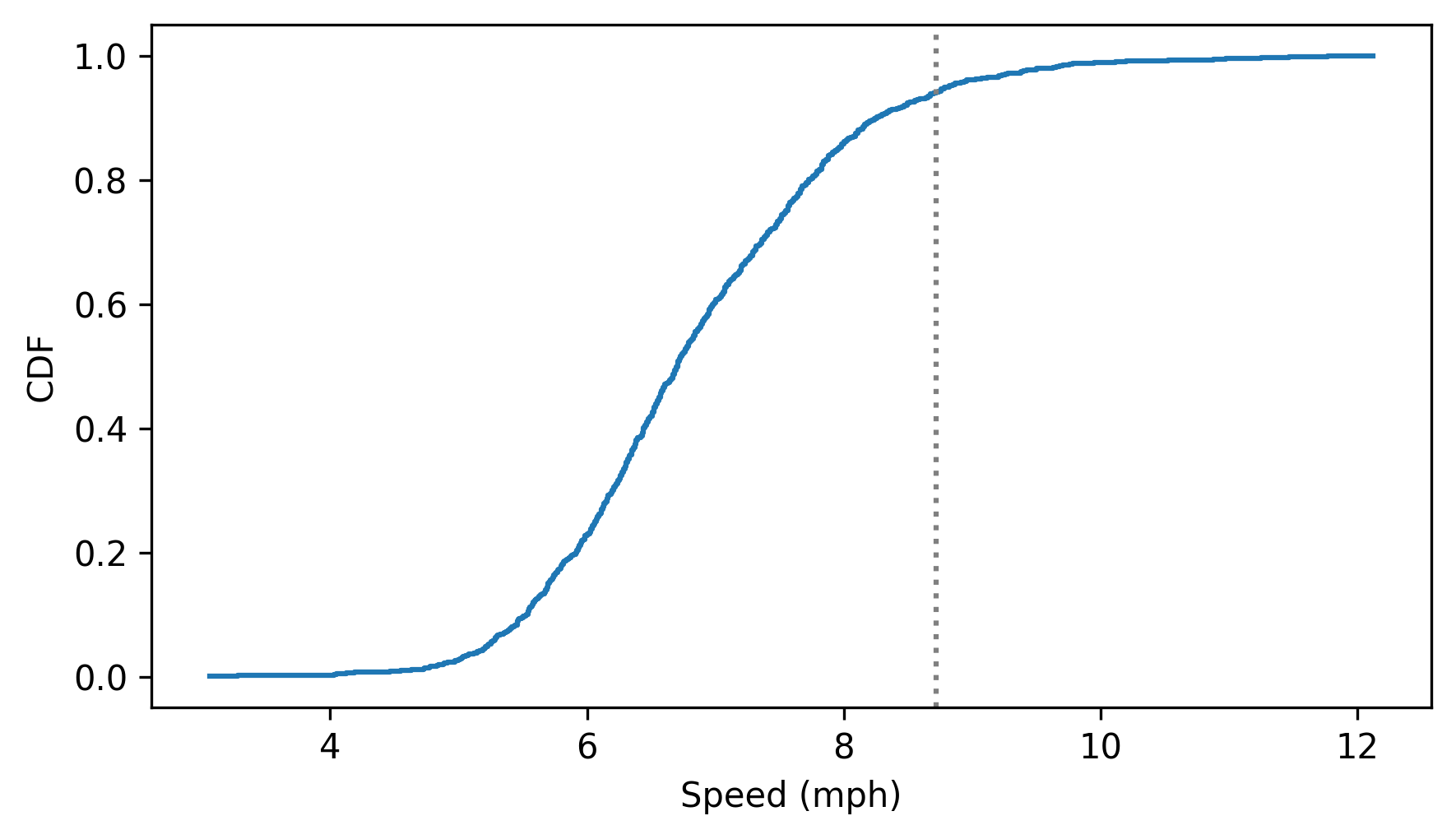
If we look up my speed, the result is the fraction of runners at my speed or slower. If we multiply by 100, we get my percentile rank.
$ cdf_speeds(my_speed) * 100
np.float64(94.12124923453766)
So that’s one way to think about the
Cdf — given a value, it computes something like a percentile rank, except that it’s a proportion between 0 and 1 rather than a percentage between 0 and 100.
Cdf provides an inverse method that computes the inverse of the cumulative distribution function — given a proportion between 0 and 1, it finds the corresponding value.
For example, if someone says they ran as fast or faster than 50% of the field, we can find their speed like this.
$ cdf_speeds.inverse(0.5)
array(6.70391061)
If you have a proportion and you use the inverse CDF to find the corresponding value, the result is called a quantile — so the inverse CDF is sometimes called the quantile function.
If you have a quantile and you use the CDF to find the corresponding proportion, the result doesn’t really have a name, strangely. To be consistent with percentile and percentile rank, it could be called a "quantile rank", but as far as I can tell, no one calls it that. Most often, it is just called a "cumulative probability".

