Section 5.1 The Binomial Distribution
As a first example, we’ll consider the sport of skeet shooting, in which competitors use shotguns to shoot clay disks that are thrown into the air. In international competition, including the Olympics, there are five rounds with 25 targets per round, with additional rounds as needed to determine a winner.
As a model of a skeet-shooting competition, suppose that every participant has the same probability,
p, of hitting every target. Of course, this model is a simplification — in reality, some competitors have a higher probability than others, and even for a single competitor, it might vary from one attempt to the next. But even if it is not realistic, this model makes some surprisingly accurate predictions, as we’ll see.
To simulate the model, I’ll use the following function, which takes the number of targets,
n, and the probability of hitting each one, p, and returns a sequence of 1s and 0s to indicate hits and misses.
def flip(n, p):
    choices = [1, 0]
    probs = [p, 1 - p]
    return np.random.choice(choices, n, p=probs)
Here’s an example that simulates a round of 25 targets where the probability of hitting each one is 90%.
# Seed the random number generator so we get the same results every time
np.random.seed(1)
$ flip(25, 0.9)
array([1, 1, 1, 1, 1, 1, 1, 1, 1, 1, 1, 1, 1, 1, 1, 1, 1, 1, 1, 1, 1, 0,
       1, 1, 1])
If we generate a longer sequence and compute the
Pmf of the results, we can confirm that the proportions of 1s and 0s are correct, at least approximately.
$ from empiricaldist import Pmf

seq = flip(1000, 0.9)
pmf = Pmf.from_seq(seq)
pmf
0    0.101
1    0.899
Name: , dtype: float64
Now we can use
flip to simulate a round of skeet shooting and return the number of hits.
def simulate_round(n, p):
    seq = flip(n, p)
    return seq.sum()
In a large competition, suppose 200 competitors shoot 5 rounds each, all with the same probability of hitting the target,
p=0.9. We can simulate a competition like that by calling simulate_round 1000 times.
n = 25
p = 0.9
results_sim = [simulate_round(n, p) for i in range(1000)]
$ np.mean(results_sim), n * p
(np.float64(22.522), 22.5)
Here’s what the distribution of the results looks like.
from empiricaldist import Pmf

pmf_sim = Pmf.from_seq(results_sim, name="simulation results")

pmf_sim.bar()
decorate(xlabel="Hits", ylabel="PMF")
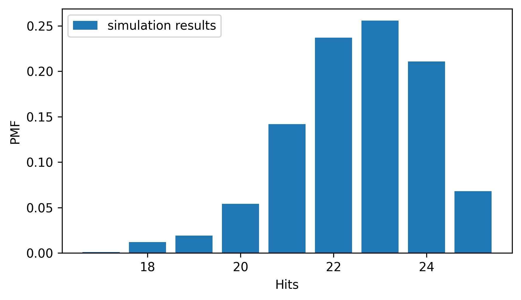
The peak is near the mean, and the distribution is skewed to the left.
Instead of running a simulation, we could have predicted this distribution. Mathematically, the distribution of these outcomes follows a binomial distribution, which has a PMF that is easy to compute.
from scipy.special import comb


def binomial_pmf(k, n, p):
    return comb(n, k) * (p**k) * ((1 - p) ** (n - k))
SciPy provides the
comb function, which computes the number of combinations of n things taken k at a time, often pronounced "n choose k".
binomial_pmf computes the probability of getting k hits out of n attempts, given p. If we call this function with a range of k values, we can make a Pmf that represents the distribution of the outcomes.
ks = np.arange(16, n + 1)
ps = binomial_pmf(ks, n, p)
pmf_binom = Pmf(ps, ks, name="binomial model")
And here’s what it looks like compared to the simulation results.
from thinkstats import two_bar_plots

two_bar_plots(pmf_sim, pmf_binom)
decorate(xlabel="Hits", ylabel="PMF")
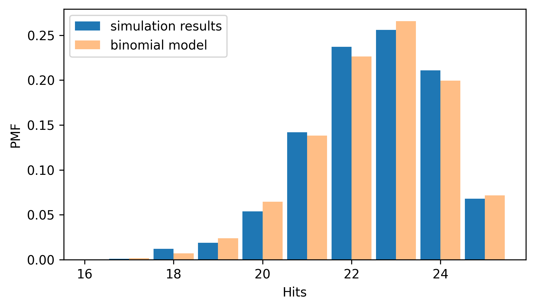
They are similar, with small differences because of random variation in the simulation results. This agreement should not be surprising, because the simulation and the model are based on the same assumptions — particularly the assumption that every attempt has the same probability of success. A stronger test of a model is how it compares to real data.
From the Wikipedia page for the men’s skeet shooting competition at the 2020 Summer Olympics, we can extract a table that shows the results for the qualification rounds.
Downloaded from https://en.wikipedia.org/wiki/Shooting_at_the_2020_Summer_Olympics_–_Men’s_skeet on July 15, 2024.
filename = "Shooting_at_the_2020_Summer_Olympics_Mens_skeet"
download("https://github.com/AllenDowney/ThinkStats/raw/v3/data/" + filename)
$ tables = pd.read_html(filename)
table = tables[6]
table.head()
   Rank              Athlete        Country   1   2   3   4   5 Total[3]  \
0     1        Éric Delaunay         France  25  25  25  24  25      124
1     2    Tammaro Cassandro          Italy  24  25  25  25  25      124
2     3      Eetu Kallioinen        Finland  25  25  24  25  24      123
3     4      Vincent Hancock  United States  25  25  25  25  22      122
4     5  Abdullah Al-Rashidi         Kuwait  25  25  24  25  23      122

   Shoot-off  Notes
0        +6  Q, OR
1        +5  Q, OR
2       NaN      Q
3        +8      Q
4        +7      Q
The table has one row for each competitor, with one column for each of five rounds. We’ll select the columns that contain these results and use the NumPy function
flatten to put them into a single array.
columns = ["1", "2", "3", "4", "5"]
results = table[columns].values.flatten()
With 30 competitors, we have results from 150 rounds of 25 shots each, with 3750 hits out of a total of 3575 attempts.
$ total_shots = 25 * len(results)
total_hits = results.sum()
n, total_shots, total_hits
(25, 3750, np.int64(3575))
So the overall success rate is 95.3%.
$ p = total_hits / total_shots
p
np.float64(0.9533333333333334)
Now let’s compute a
Pmf that represents the binomial distribution with n=25 and the value of p we just computed, and compare that to the Pmf of the actual results.
ps = binomial_pmf(ks, n, p)
pmf_binom = Pmf(ps, ks, name="binomial model")
pmf_results = Pmf.from_seq(results, name="actual results")

two_bar_plots(pmf_results, pmf_binom)
decorate(xlabel="Hits", ylabel="PMF")
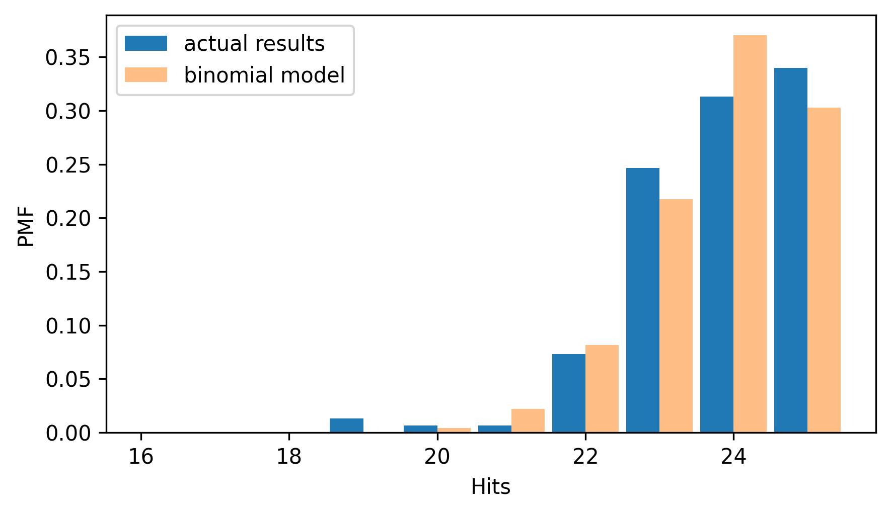
The binomial model is a good fit for the distribution of the data — even though it makes the unrealistic assumption that all competitors have the same, unchanging capability.

