Control Variables

Section 11.3 Control Variables

In Chapter 4 we saw that first babies are lighter than other babies, on average. And in Chapter 9 we saw that birth weight is correlated with the mother’s age -- older mothers have heavier babies on average.

🔗

These results might be related. If mothers of first babies are younger than mothers of other babies -- which seems likely -- that might explain why their babies are lighter. We can use multiple regression to test this conjecture, by estimating the difference in birth weight between first babies and others while controlling for the mothers’ ages.

🔗

Instructions for downloading the NSFG data are in the notebook for this chapter.

🔗

The following cells download the data files and install statadict, which we need to read the data.

🔗

Listing 11.3.1. Python Code

🔗

download("https://github.com/AllenDowney/ThinkStats/raw/v3/nb/nsfg.py")
download("https://github.com/AllenDowney/ThinkStats/raw/v3/data/2002FemPreg.dct")
download("https://github.com/AllenDowney/ThinkStats/raw/v3/data/2002FemPreg.dat.gz")

Listing 11.3.2. Python Code

🔗

try:
    import statadict
except ImportError:
    %pip install statadict

We can use get_nsfg_groups to read the data, select live births, and group live births into first babies and others.

🔗

Listing 11.3.3. Python Code

🔗

from nsfg import get_nsfg_groups

live, firsts, others = get_nsfg_groups()

We’ll use dropna to select the rows with valid birth weights, birth order, and mother’s ages.

🔗

Listing 11.3.4. Python Code

🔗

valid = live.dropna(subset=["agepreg", "birthord", "totalwgt_lb"]).copy()

Now we can use StatsModels to confirm that birth weight is correlated with age, and to estimate the slope -- assuming that it is a linear relationship.

🔗

Listing 11.3.5. Python Code

🔗

formula = "totalwgt_lb ~ agepreg"
result_age = smf.ols(formula, data=valid).fit()
display_summary(result_age)

Table 11.3.6.

🔗

	coef	std err	t	P>\|t\|	[0.025	0.975]
Intercept	6.8304	0.068	100.470	0.000	6.697	6.964
agepreg	0.0175	0.003	6.559	0.000	0.012	0.023

Table 11.3.7.

🔗

R-squared:

0.004738

The slope is small, only 0.0175 pounds per year. So if two mothers differ in age by a decade, we expect their babies to differ in weight by 0.175 pounds. But the p-value is small, so this slope -- small as it is -- would be unlikely if there were actually no relationship.

🔗

The \(R^2\) value is also small, which means that mother’s age is not very useful as a predictive variable. If we know the mother’s age, our ability to predict the baby’s weight is hardly improved at all.

🔗

This combination of a small p-value and a small \(R^2\) value is a common source of confusion, because it seems contradictory -- if the relationship is statistically significant, it seems like it should be predictive. But this example shows that there is no contradiction -- a relationship can be statistically significant but not very useful for prediction. If we visualize the results, we’ll see why. First let’s select the relevant columns.

🔗

Listing 11.3.8. Python Code

🔗

totalwgt = valid["totalwgt_lb"]
agepreg = valid["agepreg"]

To compute the fitted line, we could extract the intercept and slope from result_age, but we don’t have to. The RegressionResults object provides a predict method we can use instead. First we’ll compute a range of values for agepreg.

🔗

Listing 11.3.9. Python Code

🔗

agepreg_range = np.linspace(agepreg.min(), agepreg.max())

To use predict, we have to put values for the explanatory variables in a DataFrame.

🔗

Listing 11.3.10. Python Code

🔗

df = pd.DataFrame({"agepreg": agepreg_range})

The columns in the DataFrame have to have the same names as the explanatory variables. Then we can pass it to predict.

🔗

Listing 11.3.11. Python Code

🔗

fit_ys = result_age.predict(df)

The result is a Series containing the predicted values. Here’s what they look like, along with a scatter plot of the data.

🔗

Listing 11.3.12. Python Code

🔗

plt.scatter(agepreg, totalwgt, marker=".", alpha=0.1, s=5)
plt.plot(agepreg_range, fit_ys, color="C1", label="linear model")

decorate(xlabel="Maternal age", ylabel="Birth weight (pounds)")

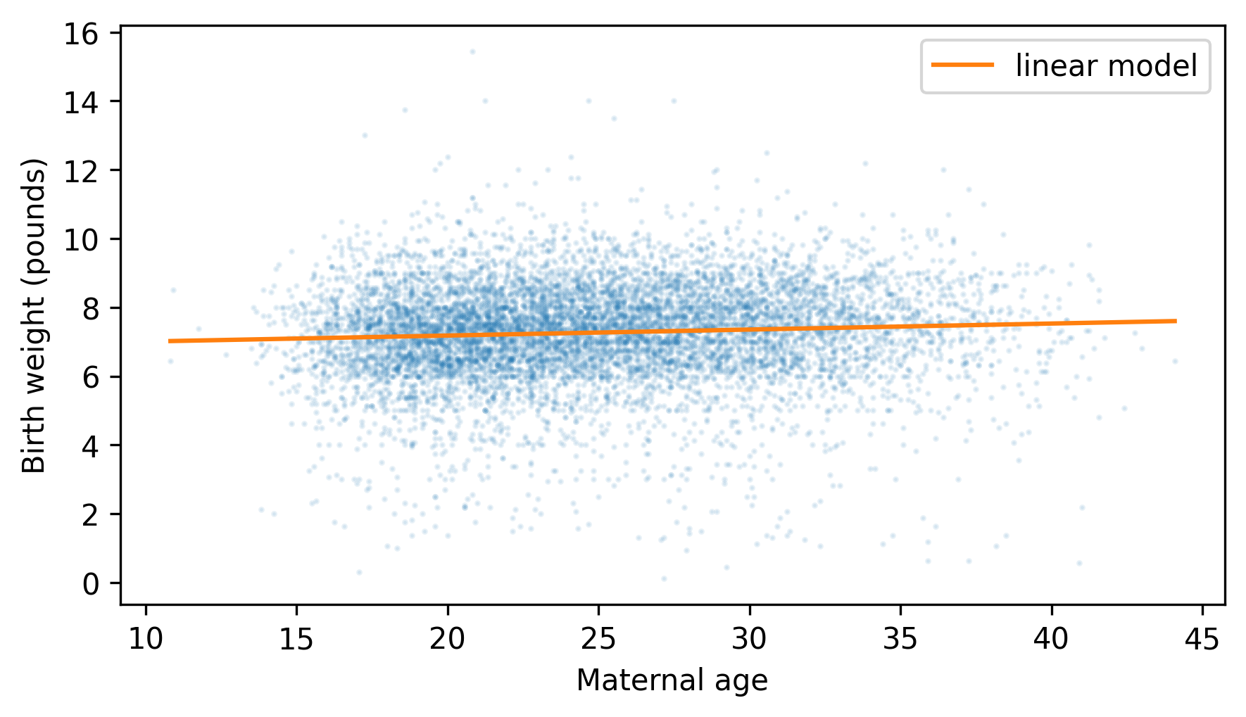
Because the slope of the fitted line is small, we can barely see the difference in the expected birth weight between the youngest and oldest mothers. The variation in birth weight, at every maternal age, is much larger.

🔗

Next we’ll use StatsModels to confirm that first babies are lighter than others. To make that work, we’ll create a Boolean Series that is True for first babies and False for others, and add it as a new column called is_first.

🔗

Listing 11.3.14. Python Code

🔗

valid["is_first"] = valid["birthord"] == 1

Listing 11.3.15. Python Code

🔗

$ from thinkstats import value_counts

# check the results
value_counts(valid["is_first"])
is_first
False    4675
True     4363
Name: count, dtype: int64

Here’s the formula for a model with birth weight as the response variable and is_first as the explanatory variable. In the Patsy formula language, C and the parentheses around the variable name indicate that it is categorical -- that is, it represents categories like "first baby" rather than measurements like birth weight.

🔗

Listing 11.3.16. Python Code

🔗

formula = "totalwgt_lb ~ C(is_first)"

Now we can fit the model and display the results, as usual.

🔗

Listing 11.3.17. Python Code

🔗

result_first = smf.ols(formula, data=valid).fit()
display_summary(result_first)

Table 11.3.18.

🔗

	coef	std err	t	P>\|t\|	[0.025	0.975]
Intercept	7.3259	0.021	356.007	0.000	7.286	7.366
C(is_first)[T.True]	-0.1248	0.030	-4.212	0.000	-0.183	-0.067

Table 11.3.19.

🔗

R-squared:

0.00196

In the results, the label C(is_first)[T.True] indicates that is_first is a categorical variable and the coefficient is associated with the value True. The T before True stands for "treatment" -- in the language of a controlled experiment, first babies are considered the treatment group and other babies are considered the reference group. These designations are arbitrary -- we could consider first babies to be the reference group and others to be the treatment group. But we need to know which is which in order to interpret the results.

🔗

The intercept is about 7.3, which means that the average weight of the reference group is 7.3 pounds. The coefficient of is_first is -0.12, which means that the average weight of the treatment group -- first babies -- is 0.12 pounds lighter. We can check both of these results by computing them directly.

🔗

Listing 11.3.20. Python Code

🔗

$ others["totalwgt_lb"].mean()
np.float64(7.325855614973262)

Listing 11.3.21. Python Code

🔗

$ diff_weight = firsts["totalwgt_lb"].mean() - others["totalwgt_lb"].mean()
diff_weight
np.float64(-0.12476118453549034)

In addition to these coefficients, StatsModels also computes p-values, confidence intervals, and \(R^2\text{.}\) The p-value associated with first babies is small, which means that the difference between the groups is statistically significant. And the \(R^2\) value is small, which means that if we’re trying to guess the weight of a baby, it doesn’t help much to know whether it is a first baby.

🔗

Now let’s see if it’s plausible that the difference in birth weight is due to the difference in maternal age. On average, mothers of first babies are about 3.6 years younger than other mothers.

🔗

Listing 11.3.22. Python Code

🔗

$ diff_age = firsts["agepreg"].mean() - others["agepreg"].mean()
diff_age
np.float64(-3.5864347661500275)

And the slope of birth weight as a function of age is 0.0175 pounds per year.

🔗

Listing 11.3.23. Python Code

🔗

$ slope = result_age.params["agepreg"]
slope
np.float64(0.017453851471802638)

If we multiply the slope by the difference in ages, we get the expected difference in birth weight for first babies and others, due to mother’s age.

🔗

Listing 11.3.24. Python Code

🔗

$ slope * diff_age
np.float64(-0.0625970997216918)

The result is 0.063 pounds, which is about half of the observed difference. So it seems like the observed difference in birth weight can be partly explained by the difference in mother’s age.

🔗

Using multiple regression, we can estimate coefficients for maternal age and first babies at the same time.

🔗

Listing 11.3.25. Python Code

🔗

formula = "totalwgt_lb ~ agepreg + C(is_first)"
result = smf.ols(formula, data=valid).fit()
display_summary(result)

Table 11.3.26.

🔗

	coef	std err	t	P>\|t\|	[0.025	0.975]
Intercept	6.9142	0.078	89.073	0.000	6.762	7.066
C(is_first)[T.True]	-0.0698	0.031	-2.236	0.025	-0.131	-0.009
agepreg	0.0154	0.003	5.499	0.000	0.010	0.021

Table 11.3.27.

🔗

R-squared:

0.005289

The coefficient of is_first is -0.0698, which means that first babies are 0.0698 pounds lighter than others, on average, after accounting for the difference due to maternal age. That’s about half of the difference we get without accounting for maternal age.

🔗

And the p-value is 0.025, which is still considered statistically significant, but it is in the borderline range where we can’t exclude the possibility that a difference this size could happen by chance.

🔗

Because this model takes into account the weight difference due to maternal age, we can say that it controls for maternal age. But it assumes that the relationship between weight and maternal age is linear. So let’s see if that’s true.

🔗

Prev Top Next