Kernel Density Estimation

Section 6.5 Kernel Density Estimation

Instead of using the model to make a PMF, we can use the data to make a PDF. To show how that works, I’ll start with a small sample of the data.

🔗

Listing 6.5.1. Python Code

🔗

# Set the random seed so we get the same results every time
np.random.seed(3)

Listing 6.5.2. Python Code

🔗

n = 10
sample = birth_weights.sample(n)

The Pmf of this sample looks like this.

🔗

Listing 6.5.3. Python Code

🔗

for weight in sample:
    pmf = Pmf.from_seq([weight]) / n
    pmf.bar(width=0.08, alpha=0.5)

xlim = [1.5, 12.5]
decorate(xlabel="Birth weight (pounds)", ylabel="PMF", xlim=xlim)

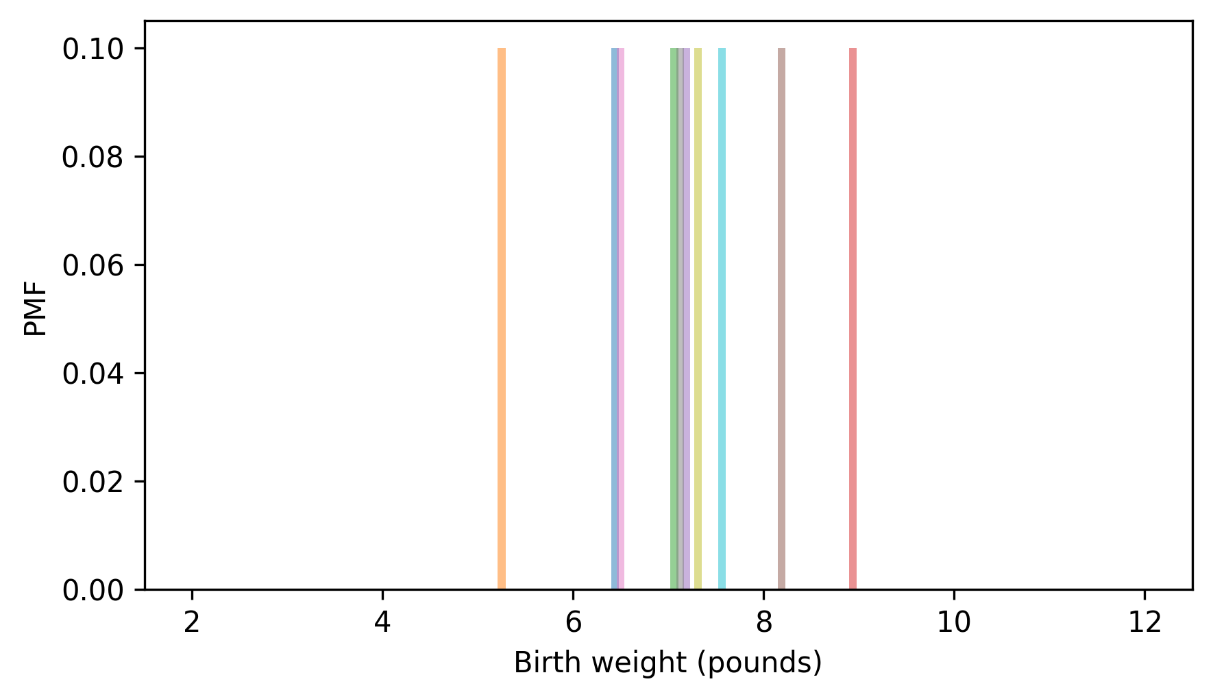
This way of representing the distribution treats the data as if it is discrete, so each probability mass is stacked up on a single point. But birth weight is actually continuous, so the quantities between the measurements are also possible. We can represent that possibility by replacing each discrete probability mass with a continuous probability density, like this.

🔗

Listing 6.5.5. Python Code

🔗

qs = np.linspace(2, 12, 201)

for weight in sample:
    ps = NormalPdf(weight, 0.75)(qs) / n
    plt.plot(qs, ps, alpha=0.5)

decorate(xlabel="Birth weight (pounds)", ylabel="PDF", xlim=xlim)

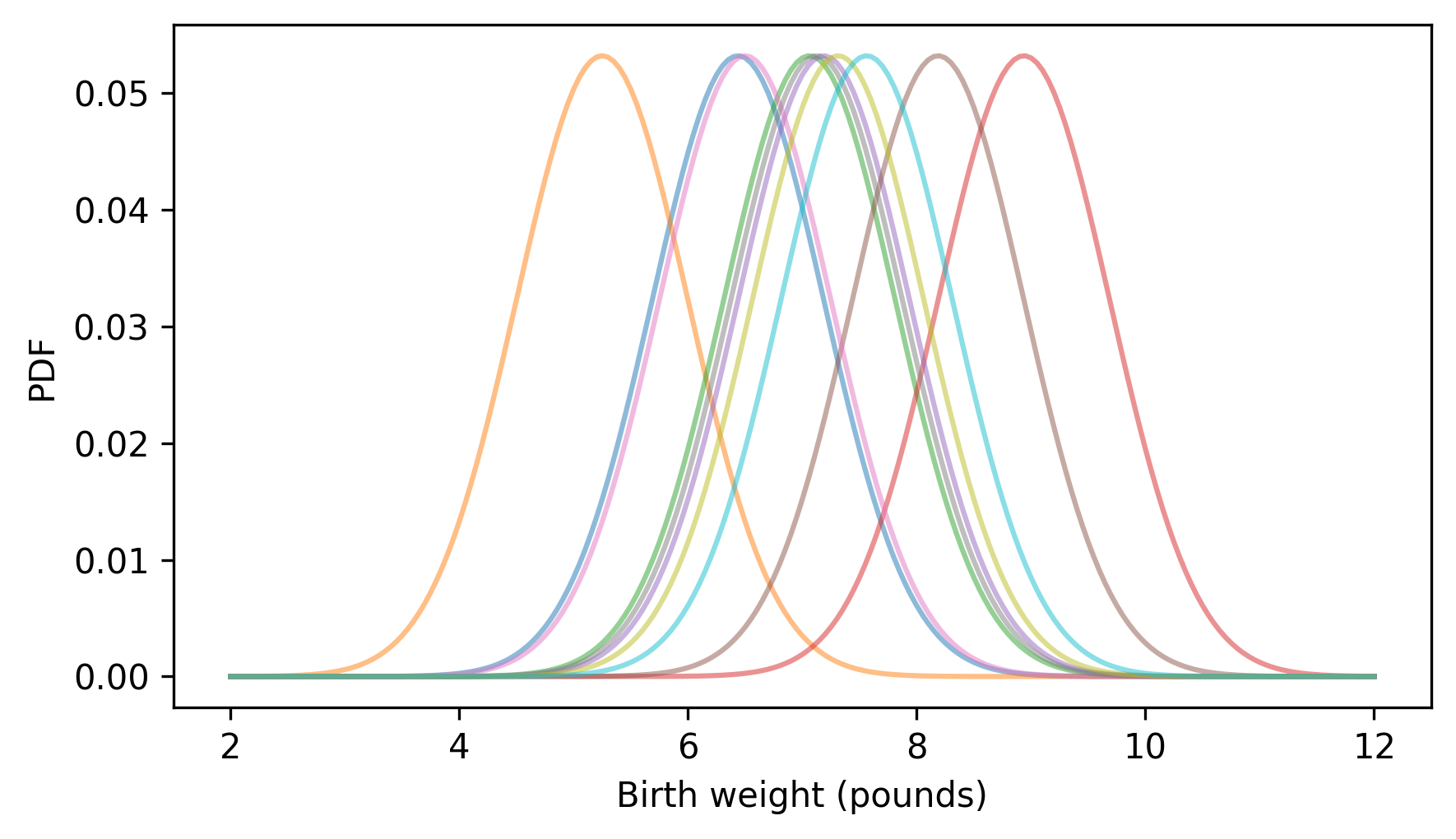
For each weight in the sample, we create a NormalPdf with the observed weight as the mean — now let’s add them up.

🔗

Listing 6.5.7. Python Code

🔗

low_ps = np.zeros_like(qs)

for weight in sample:
    ps = NormalPdf(weight, 0.75)(qs) / n
    high_ps = low_ps + ps
    plt.fill_between(qs, low_ps, high_ps, alpha=0.5, lw=1, ec="white")
    low_ps = high_ps

decorate(xlabel="Birth weight (pounds)", ylabel="PDF", xlim=xlim)

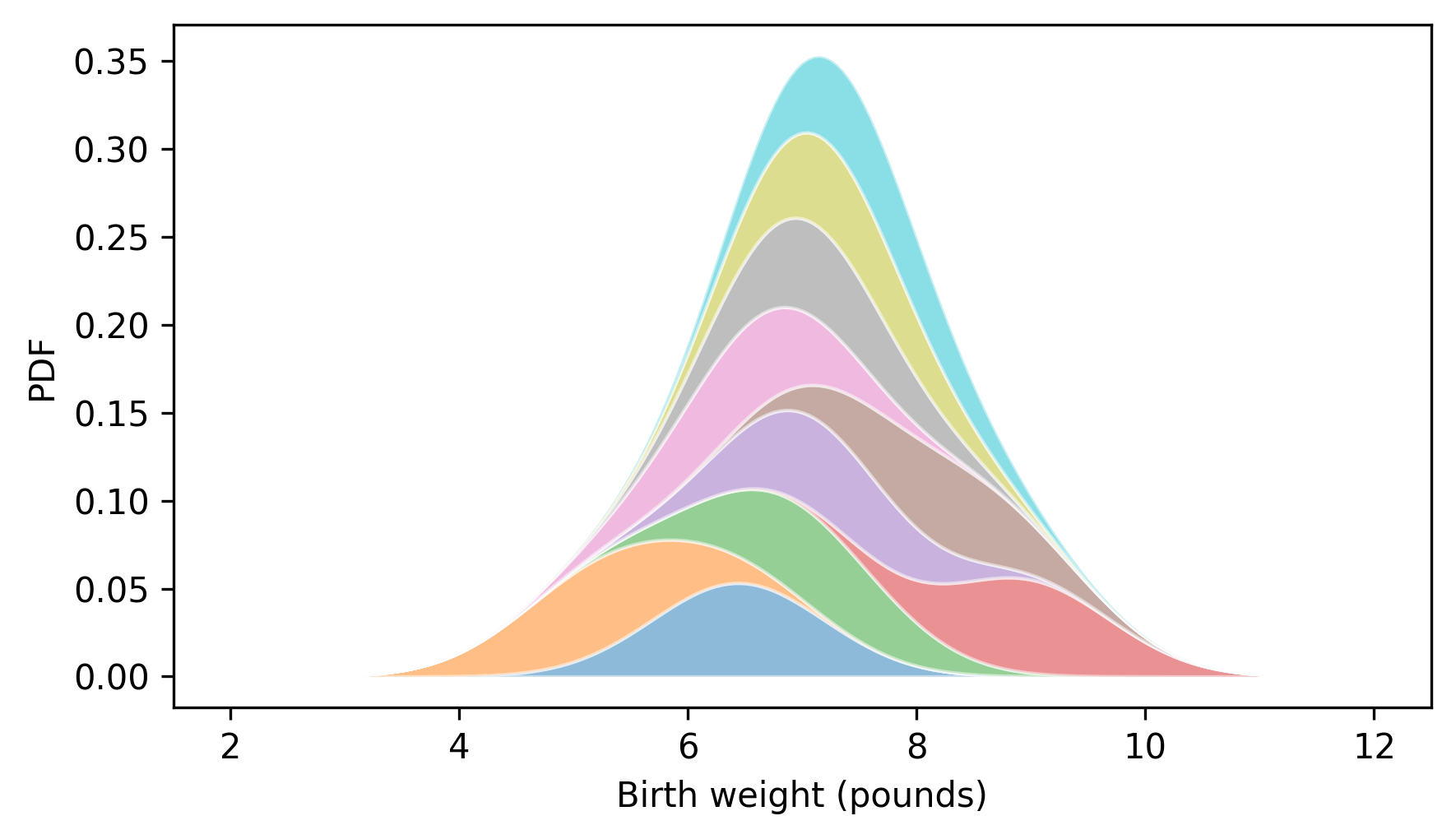
When we add up the probability densities for each data point, the result is an estimate of the probability density for the whole sample. This process is called kernel density estimation or KDE. In this context, a "kernel" is one of the small density functions we added up. Because the kernels we used are normal distributions — also known as Gaussians — we could say more specifically that we computed a Gaussian KDE.

🔗

SciPy provides a function called gaussian_kde that implements this algorithm. Here’s how we can use it to estimate the distribution of birth weights.

🔗

Listing 6.5.9. Python Code

🔗

from scipy.stats import gaussian_kde

kde = gaussian_kde(birth_weights)

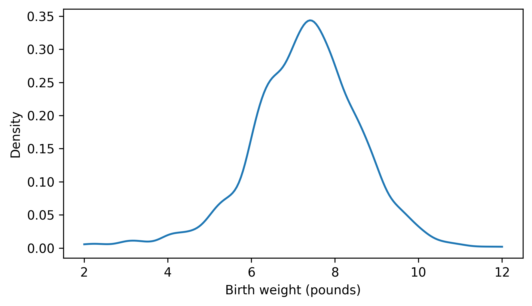
The result is an object that represents the estimated PDF, which we can evaluate by calling it like a function.

🔗

Listing 6.5.10. Python Code

🔗

ps = kde(qs)

Here’s what the result looks like.

🔗

Listing 6.5.11. Python Code

🔗

plt.plot(qs, ps)

decorate(xlabel="Birth weight (pounds)", ylabel="Density")

thinkstats provides a Pdf object that takes the result from gaussian_kde, and a domain that indicates where the density should be evaluated. Here’s how we make one.

🔗

Listing 6.5.13. Python Code

🔗

from thinkstats import Pdf

domain = np.min(birth_weights), np.max(birth_weights)
kde_birth_weights = Pdf(kde, domain, name="data")

Pdf provides a plot method we can use to compare the estimated PDF of the sample to the PDF of a normal distribution.

🔗

Listing 6.5.14. Python Code

🔗

pdf_model.plot(ls=":", color="gray")
kde_birth_weights.plot()

decorate(xlabel="Birth weight (pounds)", ylabel="Density")

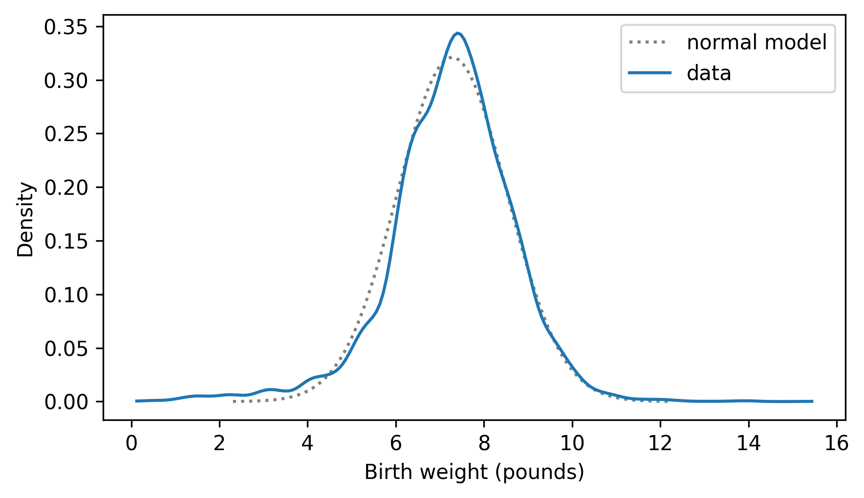
Kernel density estimation makes it possible to compare the distribution of a dataset to a theoretical model, and for some audiences, this is a good way to visualize the comparison. But for audiences that are familiar with CDFs, comparing CDFs is often better.

🔗

Prev Top Next