Section 6.3 The Exponential PDF
To get your head around probability density, it might help to see another example. In the previous chapter, we used an exponential distribution to model the time until the first goal in a hockey game. We used the following function to compute the exponential CDF, where
lam is the rate in goals per unit of time.
def exponential_cdf(x, lam):
    """Compute the exponential CDF.

    x: float or sequence of floats
    lam: rate parameter

    returns: float or NumPy array of cumulative probability
    """
    return 1 - np.exp(-lam * x)
We can compute the PDF of the exponential distribution like this.
def exponential_pdf(x, lam):
    """Evaluates the exponential PDF.

    x: float or sequence of floats
    lam: rate parameter

    returns: float or NumPy array of probability density
    """
    return lam * np.exp(-lam * x)
thinkstats provides an ExponentialPdf object that uses this function to compute the exponential PDF. We can use one to represent an exponential distribution with rate 6 goals per game.
$ from thinkstats import ExponentialPdf

lam = 6
pdf_expo = ExponentialPdf(lam, name="exponential model")
pdf_expo
ExponentialPdf(6, name='exponential model')
ExponentialPdf provides a plot function we can use to plot the PDF — notice that the unit of time is games here, rather than seconds as in the previous chapter.
qs = np.linspace(0, 1.5, 201)
pdf_expo.plot(qs, ls=":", color="gray")
decorate(xlabel="Time (games)", ylabel="Density")
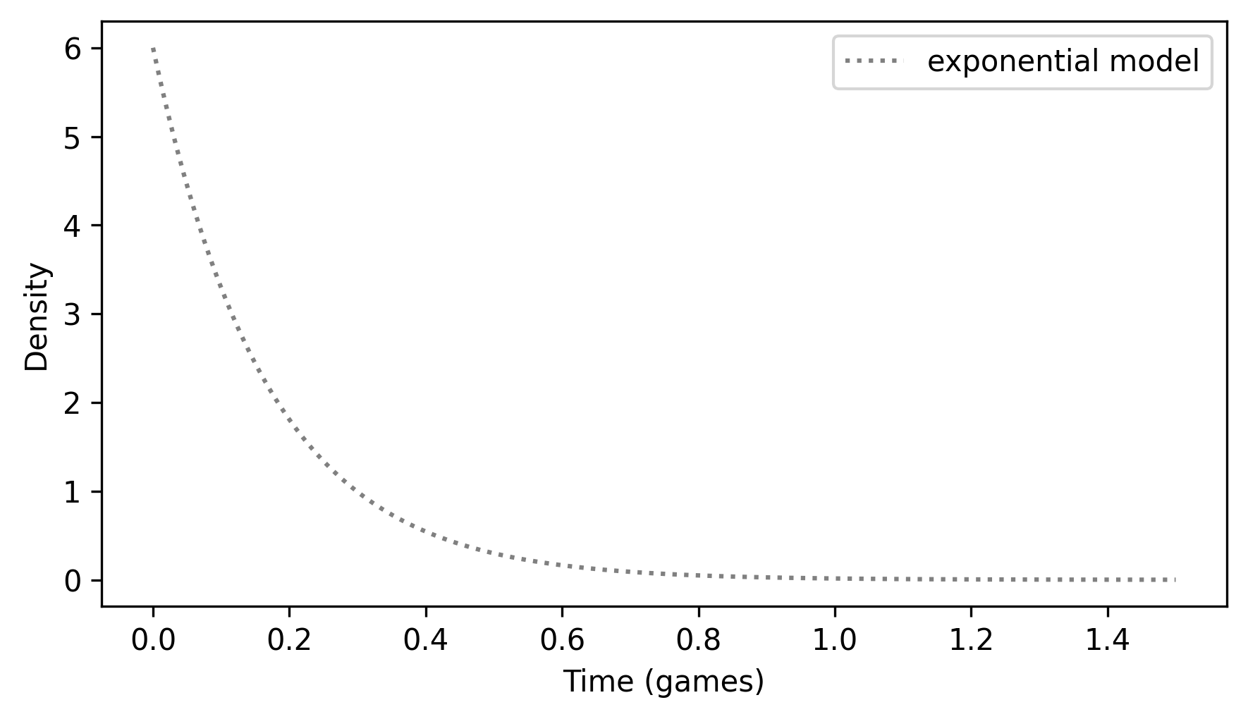
Looking at the y-axis, you might notice that some of these densities are greater than 1, which is a reminder that a probability density is not a probability. But the area under a density curve is a probability, so it should never be greater than 1.
If we compute the area under this curve from 0 to 1.5 games, we can confirm that the result is close to 1.
$ area_under(pdf_expo, 0, 1.5)
np.float64(0.999876590779019)
If we extend the interval much farther, the result is slightly greater than 1, but that’s because we’re approximating the area numerically. Mathematically, it is exactly 1, as we can confirm using the exponential CDF.
$ from thinkstats import exponential_cdf

exponential_cdf(7, lam)
np.float64(1.0)
We can use the area under the density curve to compute the probability of a goal during any interval. For example, here is the probability of a goal during the first minute of a 60-minute game.
$ area_under(pdf_expo, 0, 1 / 60)
np.float64(0.09516258196404043)
We can compute the same result using the exponential CDF.
$ exponential_cdf(1 / 60, lam)
np.float64(0.09516258196404048)
In summary, if we evaluate a PDF, the result is a probability density — which is not a probability. However, if we compute the area under the PDF, the result is the probability that a quantity falls in an interval. Or we can find the same probability by evaluating the CDF at the beginning and end of the interval and computing the difference.

