Section 14.4 Distribution of Differences
Putting together the steps from the previous section, here’s how we can compute the distribution of sample means for the weights of the female penguins.
$ n = len(weights_female)
dist_mean_female = dist_female.sum(n) / n
dist_mean_female
Normal(3368.835616438356, 994.0498530055667)
Now we have sampling distributions for the average weight of male and female penguins—let’s compute the distribution of the differences. The following method computes the distribution of the difference between values from two normal distributions.
%%add_method_to Normal


def __sub__(self, other):
    """Compute the distribution of a difference."""
    return Normal(self.mu - other.mu, self.sigma2 + other.sigma2)
As you might expect, the mean of the differences is the difference of the means. But as you might not expect, the variance of the differences is not the difference of the variances—it’s the sum! To see why, imagine we perform subtraction in two steps:
-
If we negate the second distribution, the mean is negated but the variance is the same.
-
Then if we add in the first distribution, the variance of the sum is the sum of the variances.
If that doesn’t convince you, let’s test it. Here’s the analytic distribution of the differences.
$ dist_diff_means = dist_mean_male - dist_mean_female
dist_diff_means
Normal(674.6575342465753, 2641.697160192656)
And here’s a random sample of differences.
sample_sums_female = [dist_female.sample(n).sum() for i in range(1001)]
sample_means_female = np.array(sample_sums_female) / n
sample_diff_means = sample_means_male - sample_means_female
The following figure shows the empirical CDF of the random sample and the analytic CDF of the normal distribution.
dist_diff_means.plot_cdf(**model_options)
Cdf.from_seq(sample_diff_means).plot(label="sample")

decorate(xlabel="Difference in average weight (g)", ylabel="CDF")
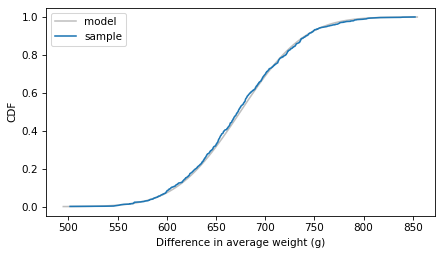
They agree, which confirms that we found the distribution of the differences correctly. We can use this distribution to compute a confidence interval for the difference in weights. We’ll use the following method to compute the inverse CDF.
%%add_method_to Normal


def ppf(self, xs):
    sigma = np.sqrt(self.sigma2)
    return norm.ppf(xs, self.mu, sigma)
The 5th and 95th percentiles form a 90% confidence interval.
$ ci90 = dist_diff_means.ppf([0.05, 0.95])
ci90
array([590.1162635 , 759.19880499])
We get approximately the same results from the random sample.
$ np.percentile(sample_diff_means, [5, 95])
array([590.86245503, 762.96045373])
The analytic method is faster than resampling, and it is deterministic—that is, not random.
However, everything we’ve done so far is based on the assumption that the distribution of measurements is normal. That’s not always true—in fact, with real data it is never exactly true. But even if the distribution of the measurements isn’t normal, if we add up many measurements, the distribution of their sum is often close to normal. That is the power of the Central Limit Theorem.

