1. Exercise 12.1.
As an example of seasonal decomposition, let’s model monthly average surface temperatures in the United States. We’ll use a dataset from Our World in Data that includes "temperature [in Celsius] of the air measured 2 meters above the ground, encompassing land, sea, and in-land water surfaces," for most countries in the world from 1950 to 2024. Instructions for downloading the data are in the notebook for this chapter.
# The following cell downloads data prepared by Our World in Data,
# which I Downloaded September 18, 2024
# from https://ourworldindata.org/grapher/average-monthly-surface-temperature

# Based on modified data from Copernicus Climate Change Service information (2019)
# with "major processing" by Our World in Data
filename = "monthly-average-surface-temperatures-by-year.csv"
download("https://github.com/AllenDowney/ThinkStats/raw/v3/data/" + filename)
We can read the data like this.
temp = pd.read_csv("monthly-average-surface-temperatures-by-year.csv")
$ temp.head()
        Entity Code  Year       2024       2023       2022       2021  \
0  Afghanistan  AFG     1   3.300064  -4.335608  -0.322859  -1.001608
1  Afghanistan  AFG     2   1.024550   4.187041   2.165870   5.688000
2  Afghanistan  AFG     3   5.843506  10.105444  10.483686   9.777976
3  Afghanistan  AFG     4  11.627398  14.277164  17.227650  15.168276
4  Afghanistan  AFG     5  18.957850  19.078170  19.962734  19.885902

        2020       2019       2018  ...       1959       1958       1956  \
0  -2.560545   0.585145   1.042471  ...  -2.333814   0.576404  -3.351925
1   2.880046   0.068664   3.622793  ...  -1.545529   0.264962   0.455350
2   6.916731   5.758049  10.794412  ...   5.942937   7.716459   5.090270
3  12.686832  13.838840  14.321226  ...  13.752827  14.712909  11.982360
4  18.884047  18.461287  18.100782  ...  17.388723  16.352045  20.125462

        1954       1952       1957       1955       1953       1951       1950
0  -2.276692  -2.812619  -4.239172  -2.191683  -2.915993  -3.126317  -2.655707
1  -0.304205   0.798226  -2.747945   1.999074   1.983414  -2.642800  -3.996040
2   4.357703   4.796146   4.434027   7.066073   4.590406   3.054388   3.491112
3  12.155265  13.119270   8.263829  10.418768  11.087193   9.682878   8.332797
4  18.432117  17.614851  15.505956  15.599709  17.865084  17.095737  17.329062

[5 rows x 78 columns]
The following cell selects data for the United States from 2001 to the end of the series and packs it into a Pandas
Series.
temp_us = temp.query("Code == 'USA'")
columns = [str(year) for year in range(2000, 2025)]
temp_series = temp_us.loc[:, columns].transpose().stack()
temp_series.index = pd.date_range(start="2000-01", periods=len(temp_series), freq="ME")
Here’s what it looks like.
temp_series.plot(label="monthly average", **actual_options)
decorate(ylabel="Surface temperature (degC)")
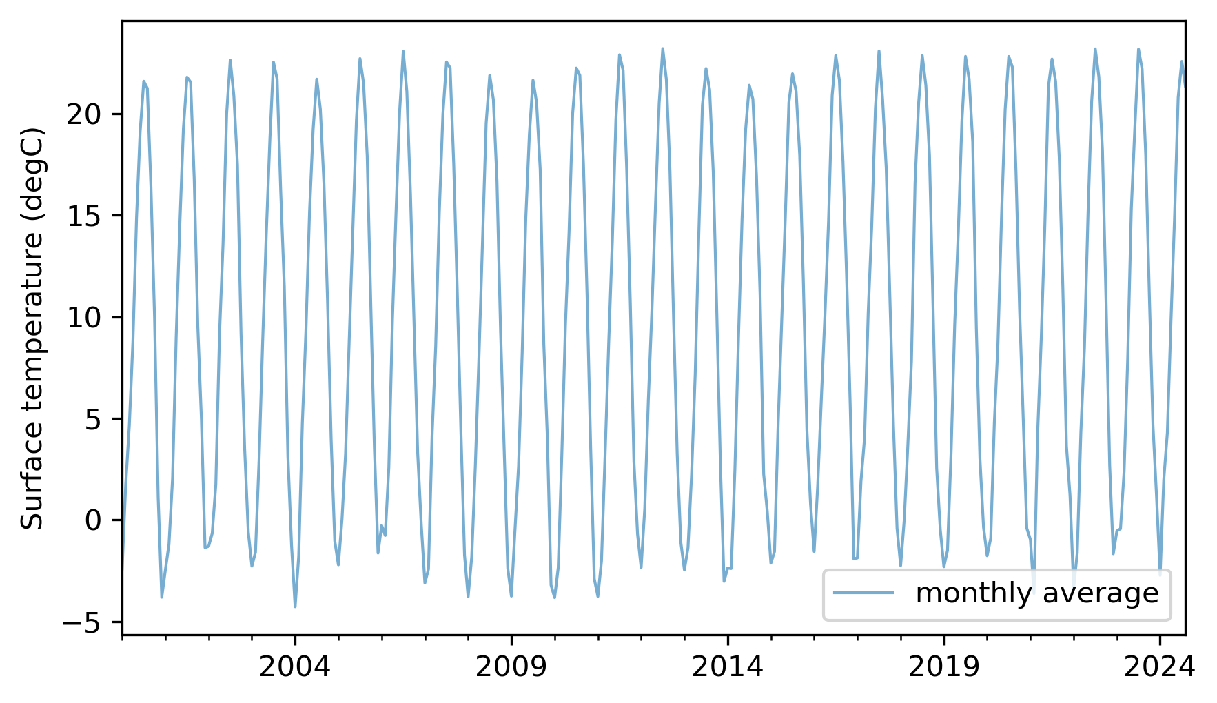
Not surprisingly, there is a strong seasonal pattern. Compute an additive seasonal decomposition with a period of 12 months. Fit a linear model to the trend line. What is the average annual increase in surface temperature during this interval? If you are curious, repeat this analysis with other intervals or data from other countries.