Logistic Regression

Section 11.5 Logistic Regression

Linear regression is based on a model where the expected value of the response variable is the weighted sum of the explanatory variables and an intercept. This model is appropriate when the response variable is a continuous quantity like birth weight or penguin mass, but not when the response variable is a discrete quantity like a count or a category.

🔗

For these kinds of response variables, we can use generalized linear models or GLMs. For example:

🔗

If the response variable is a count, we can use Poisson regression.
🔗

🔗
If it’s categorical with only two categories, we can use logistic regression.
🔗

🔗
If it’s categorical with more than two categories, we can use multinomial logistic regression.
🔗

🔗
If it’s categorical and the categories can be arranged in order, we can use ordered logistic regression.
🔗

🔗

We won’t cover all of them in this book -- just logistic regression, which is the most widely used. As an example, we’ll use the penguin dataset again, and see if we can tell whether a penguin is male or female, based on its weight and other measurements.

🔗

StatsModels provides a function that does logistic regression -- it’s called logit because that’s the name of a mathematical function that appears in the definition of logistic regression. Before we can use the logit function, we have to transform the response variable so the values are 0 and 1.

🔗

Listing 11.5.1. Python Code

🔗

adelie["y"] = (adelie["Sex"] == "MALE").astype(int)

Listing 11.5.2. Python Code

🔗

$ adelie["y"].value_counts()
y
0    78
1    73
Name: count, dtype: int64

We’ll start with a simple model with y as the response variable and mass as the explanatory variable. Here’s how we make and fit the model -- the argument disp=False suppresses messages about the fitting process.

🔗

Listing 11.5.3. Python Code

🔗

model = smf.logit("y ~ mass", data=adelie)
result = model.fit(disp=False)

And here are the results.

🔗

Listing 11.5.4. Python Code

🔗

display_summary(result)

Table 11.5.5.

🔗

	coef	std err	z	P>\|z\|	[0.025	0.975]
Intercept	-25.9871	4.221	-6.156	0.000	-34.261	-17.713
mass	0.0070	0.001	6.138	0.000	0.005	0.009

Table 11.5.6.

🔗

Pseudo R-squared:

0.5264

The coefficient of determination, \(R^2\text{,}\) does not apply to logistic regression, but there are several alternatives that are used as "pseudo \(R^2\) values." The pseudo \(R^2\) value for this model is about 0.526, which doesn’t mean much by itself, but we will use it to compare models.

🔗

The coefficient of mass is positive, which means that heavier penguins are more likely to be male. Other than that, the coefficients are not easy to interpret -- we can understand the model better by plotting the predictions. We’ll make a DataFrame with a range of values for mass, and use predict to compute a Series of predictions.

🔗

Listing 11.5.7. Python Code

🔗

mass = adelie["mass"]
mass_range = np.linspace(mass.min(), mass.max())
df = pd.DataFrame({"mass": mass_range})
fit_ys = result.predict(df)

Each predicted value is the probability a penguin is male as a function of its weight. Here’s what the predicted values look like.

🔗

Listing 11.5.8. Python Code

🔗

plt.plot(mass_range, fit_ys)

decorate(xlabel="Mass (g)", ylabel="Prob(male)")

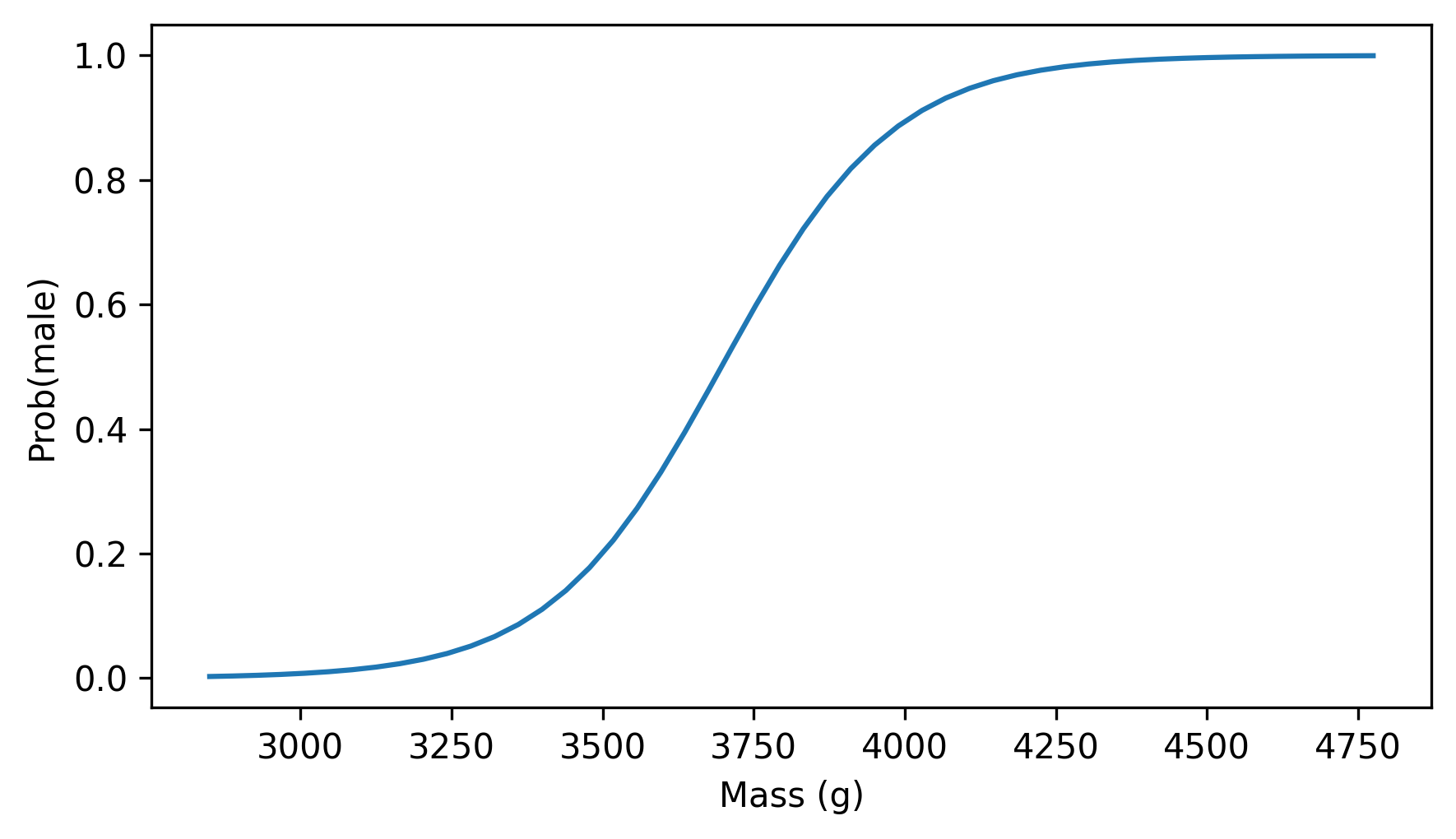
The lightest penguins are almost certain to be female, and the heaviest are likely to be male -- in the middle, a penguin weighing 3750 grams is about equally likely to be male or female.

🔗

Now let’s see what happens if we add the other measurements as explanatory variables.

🔗

Listing 11.5.10. Python Code

🔗

formula = "y ~ mass + flipper_length + culmen_length + culmen_depth"
model = smf.logit(formula, data=adelie)
result = model.fit(disp=False)
display_summary(result)

Table 11.5.11.

🔗

	coef	std err	z	P>\|z\|	[0.025	0.975]
Intercept	-60.6075	13.793	-4.394	0.000	-87.642	-33.573
mass	0.0059	0.001	4.153	0.000	0.003	0.009
flipper_length	-0.0209	0.052	-0.403	0.687	-0.123	0.081
culmen_length	0.6208	0.176	3.536	0.000	0.277	0.965
culmen_depth	1.0111	0.349	2.896	0.004	0.327	1.695

Table 11.5.12.

🔗

Pseudo R-squared:

0.6622

The pseudo \(R^2\) value of this model is 0.662, higher than the previous model (0.526) -- so the additional measurements contain additional information that distinguishes male and female penguins.

🔗

The p-values for culmen length and depth are small, which indicates that they contribute more information than we expect by chance. The p-value for flipper length is large, which suggests that if you know a penguin’s weight and bill dimensions, flipper length doesn’t contribute additional information.

🔗

To understand this model, let’s look at some of its predictions. We’ll use the following function, which takes a sequence of masses and a specific value for culmen_length. It sets the other measurements to their mean values, computes predicted probabilities as a function of mass, and plots the results.

🔗

Listing 11.5.13. Python Code

🔗

def plot_predictions(mass_range, culmen_length, **options):
    """Plot predicted probabilities as a function of mass."""
    df = pd.DataFrame({"mass": mass_range})
    df["flipper_length"] = adelie["flipper_length"].mean()
    df["culmen_length"] = culmen_length
    df["culmen_depth"] = adelie["culmen_depth"].mean()
    fit_ys = result.predict(df)
    plt.plot(mass_range, fit_ys, **options)

Here’s what the results look like for three values of culmen_length: one standard deviation above average, average, and one standard deviation below average.

🔗

Listing 11.5.14. Python Code

🔗

culmen_length = adelie["culmen_length"]
m, s = culmen_length.mean(), culmen_length.std()

Listing 11.5.15. Python Code

🔗

plot_predictions(mass_range, m + s, ls="--", label="Above average culmen length")
plot_predictions(mass_range, m, alpha=0.5, label="Average culmen length")
plot_predictions(mass_range, m - s, ls=":", label="Below average culmen length")

decorate(xlabel="Mass (g)", ylabel="Prob(male)")

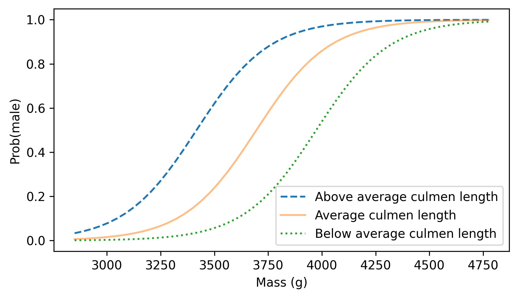
As we saw in the simpler model, heavier penguins are more likely to be male. Also, at any weight, a penguin with a longer bill is more likely to be male.

🔗

This model is more useful than it might seem -- in fact, it is similar to models that were used in the original research paper this dataset was collected for. The primary topic of that research is sexual dimorphism, which is the degree to which male and female bodies differ. One way to quantify dimorphism is to use measurements to classify males and females. In a species with higher dimorphism, we expect these classifications to be more accurate.

🔗

The original paper is Gorman KB, Williams TD, Fraser WR (2014). Ecological sexual dimorphism and environmental variability within a community of Antarctic penguins (genus Pygoscelis). PLoS ONE 9(3):e90081. https://doi.org/10.1371/journal.pone.0090081

🔗

To test this methodology, let’s try the same model on a different species. In addition to the Adélie penguins we’ve worked with so far, the dataset also contains measurements from 123 Gentoo penguins. We’ll use the following function to select them.

🔗

Listing 11.5.17. Python Code

🔗

def get_species(penguins, species):
    df = penguins.query(f'Species.str.startswith("{species}")').copy()
    df["y"] = (df["Sex"] == "MALE").astype(int)
    return df

Listing 11.5.18. Python Code

🔗

$ gentoo = get_species(penguins, "Gentoo")
len(gentoo)
123

Here are the results of the logistic regression model.

🔗

Listing 11.5.19. Python Code

🔗

formula = "y ~ mass + flipper_length + culmen_length + culmen_depth"
model = smf.logit(formula, data=gentoo)
result = model.fit(disp=False)
display_summary(result)

Table 11.5.20.

🔗

	coef	std err	z	P>\|z\|	[0.025	0.975]
Intercept	-173.9123	62.326	-2.790	0.005	-296.069	-51.756
mass	0.0105	0.004	2.948	0.003	0.004	0.017
flipper_length	0.2839	0.183	1.549	0.121	-0.075	0.643
culmen_length	0.2734	0.285	0.958	0.338	-0.286	0.833
culmen_depth	3.0843	1.291	2.389	0.017	0.554	5.614

Table 11.5.21.

🔗

Pseudo R-squared:

0.848

The pseudo-\(R^2\) value is 0.848, higher than what we got with Adélie penguins (0.662). That means Gentoo penguins can be classified more accurately using physical measurements, compared to Adélie penguins, which suggests that Gentoo penguins are more dimorphic.

🔗

Prev Top Next