Expected Remaining Lifetime

Section 13.9 Expected Remaining Lifetime

Given a distribution, we can compute the expected remaining lifetime as a function of elapsed time. For example, given the distribution of pregnancy lengths, we can compute the expected time until delivery. To demonstrate, we’ll use pregnancy data from the NSFG.

🔗

The following cells download the data files and install statadict, which we need to read the data.

🔗

Listing 13.9.1. Python Code

🔗

download("https://github.com/AllenDowney/ThinkStats/raw/v3/nb/nsfg.py")
download("https://github.com/AllenDowney/ThinkStats/raw/v3/data/2002FemPreg.dct")
download("https://github.com/AllenDowney/ThinkStats/raw/v3/data/2002FemPreg.dat.gz")

Listing 13.9.2. Python Code

🔗

try:
    import statadict
except ImportError:
    %pip install statadict

We’ll use get_nsfg_groups to read the data and divide it into first babies and others.

🔗

Listing 13.9.3. Python Code

🔗

from nsfg import get_nsfg_groups

live, firsts, others = get_nsfg_groups()

/home/runner/work/ThinkStats/ThinkStats/soln/nsfg.py:190: PerformanceWarning: DataFrame is highly fragmented.  This is usually the result of calling `frame.insert` many times, which has poor performance.  Consider joining all columns at once using pd.concat(axis=1) instead. To get a de-fragmented frame, use `newframe = frame.copy()`
  df["totalwgt_lb"] = df.birthwgt_lb + df.birthwgt_oz / 16.0

We’ll start with a single resampling of the data.

🔗

Listing 13.9.4. Python Code

🔗

sample = resample_rows_weighted(live, "finalwgt")

Here’s the PMF of pregnancy durations.

🔗

Listing 13.9.5. Python Code

🔗

pmf_durations = Pmf.from_seq(sample["prglngth"])

Now suppose it’s the beginning of the 36th week of pregnancy. Remembering that the most common pregnancy length is 39 weeks, we expect the remaining time to be 3-4 weeks. To make that estimate more precise, we can identify the values in the distribution that equal or exceed 36 weeks.

🔗

Listing 13.9.6. Python Code

🔗

t = 36
is_remaining = pmf_durations.qs >= t

Next we’ll make a new Pmf object that contains only those values, shifted left so the current time is at 0.

🔗

Listing 13.9.7. Python Code

🔗

ps = pmf_durations.ps[is_remaining]
qs = pmf_durations.qs[is_remaining] - t

pmf_remaining = Pmf(ps, qs)

Because we selected a subset of the values in the Pmf, the probabilities no longer add up to 1, but we can normalize the Pmf so they do.

🔗

Listing 13.9.8. Python Code

🔗

pmf_remaining.normalize()

np.float64(0.9155006558810669)

Here’s the result, which shows the distribution of remaining time at the beginning of the 36th week.

🔗

Listing 13.9.9. Python Code

🔗

pmf_remaining.bar(label="Week 36")
decorate(xlabel="Remaining duration (weeks)", ylabel="PMF")

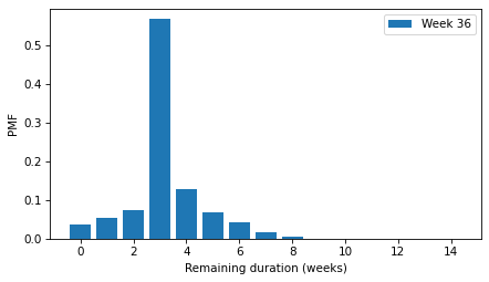
The mean of this distribution is the expected remaining time.

🔗

Listing 13.9.11. Python Code

🔗

pmf_remaining.mean()

np.float64(3.2145671641791043)

The following function encapsulates these steps and computes the distribution of remaining time for a given Pmf at a given time, t.

🔗

Listing 13.9.12. Python Code

🔗

def compute_pmf_remaining(pmf, t):
    """Distribution of remaining time."""
    is_remaining = pmf.qs >= t
    ps = pmf.ps[is_remaining]
    qs = pmf.qs[is_remaining] - t
    pmf_remaining = Pmf(ps, qs)
    pmf_remaining.normalize()
    return pmf_remaining

The following function takes a Pmf of pregnancy lengths and computes the expected remaining time at the beginning of each week from the 36th to the 43rd.

🔗

Listing 13.9.13. Python Code

🔗

def expected_remaining(pmf):
    index = range(36, 44)
    expected = pd.Series(index=index)

    for t in index:
        pmf_remaining = compute_pmf_remaining(pmf, t)
        expected[t] = pmf_remaining.mean()

    return expected

Here are the results for a single resampling of the data.

🔗

Listing 13.9.14. Python Code

🔗

expected = expected_remaining(pmf_durations)
expected

36    3.214567
37    2.337714
38    1.479095
39    0.610133
40    0.912517
41    0.784211
42    0.582301
43    0.589372
dtype: float64

To see how much variation there is due to random sampling, we can run this analysis with several resamplings and plot the results.

🔗

Listing 13.9.15. Python Code

🔗

for i in range(21):
    sample = resample_rows_weighted(live, "finalwgt")
    pmf_durations = Pmf.from_seq(sample["prglngth"])
    expected = expected_remaining(pmf_durations)
    expected.plot(color="C0", alpha=0.1)

decorate(
    xlabel="Weeks of pregnancy", ylabel="Expected remaining time (weeks)", ylim=[0, 3.4]
)

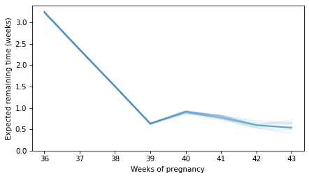
Between weeks 36 and 39, the expected remaining time decreases until, at the beginning of the 39th week, it is about 0.6 weeks. But after that, the curve levels off. At the beginning of the 40th week, the expected remaining time is still close to 0.6 weeks—actually a little higher—and at the beginning of the 41st, 42nd, and 43rd, it is almost the same. For people waiting anxiously for a baby to be born, this behavior seems quite cruel.

🔗

Prev Top Next