Section C.1 Air Temperature
In the chapter on time series analysis, in an exercise on seasonal decomposition, we use monthly average surface temperatures in the United States, from a dataset from Our World in Data that includes “temperature [in Celsius] of the air measured 2 meters above the ground, encompassing land, sea, and in-land water surfaces.”
The following code uses the API to download metadata about the dataset.
import requests

url = (
    "https://ourworldindata.org/grapher/"
    "average-monthly-surface-temperature.metadata.json"
)
query_params = {"v": "1", "csvType": "full", "useColumnShortNames": "true"}
headers = {"User-Agent": "Our World In Data data fetch/1.0"}

response = requests.get(url, params=query_params, headers=headers)
metadata = response.json()
The result is a nested dictionary. Here are the top-level keys.
$ metadata.keys()
dict_keys(['chart', 'columns', 'dateDownloaded'])
Here’s the chart-level documentation.
$ from pprint import pprint

pprint(metadata["chart"])
{'citation': 'Contains modified Copernicus Climate Change Service information '
             '(2019)',
 'originalChartUrl': 'https://ourworldindata.org/grapher/average-monthly-surface-temperature?v=1&csvType=full&useColumnShortNames=true',
 'selection': ['World'],
 'subtitle': 'The temperature of the air measured 2 meters above the ground, '
             'encompassing land, sea, and in-land water surfaces.',
 'title': 'Average monthly surface temperature'}
And here’s the documentation of the column we’ll use.
$ pprint(metadata["columns"]["temperature_2m"])
{'citationLong': 'Contains modified Copernicus Climate Change Service '
                 'information (2019) – with major processing by Our World in '
                 'Data. “Annual average” [dataset]. Contains modified '
                 'Copernicus Climate Change Service information, “ERA5 monthly '
                 'averaged data on single levels from 1940 to present 2” '
                 '[original data].',
 'citationShort': 'Contains modified Copernicus Climate Change Service '
                  'information (2019) – with major processing by Our World in '
                  'Data',
 'descriptionKey': [],
 'descriptionProcessing': '- Temperature measured in kelvin was converted to '
                          'degrees Celsius (°C) by subtracting 273.15.\n'
                          '\n'
                          '- Initially, the temperature dataset is provided '
                          'with specific coordinates in terms of longitude and '
                          'latitude. To tailor this data to each country, we '
                          'utilize geographical boundaries as defined by the '
                          'World Bank. The method involves trimming the global '
                          'temperature dataset to match the exact geographical '
                          'shape of each country. To correct for potential '
                          "distortions caused by the Earth's curvature on a "
                          'flat map, we apply a latitude-based weighting. This '
                          'step is essential for maintaining accuracy, '
                          'especially in high-latitude regions where '
                          'distortion is more pronounced. The result of this '
                          'process is a latitude-weighted average temperature '
                          'for each nation.\n'
                          '\n'
                          "- It's important to note, however, that due to the "

... (output truncated)
The following cells download the data for the United States—to see data from another country, change
country_code to almost any three-letter ISO 3166 country code.
country_code = "USA"  # replace this with other three-letter country codes
base_url = (
    "https://ourworldindata.org/grapher/"
    "average-monthly-surface-temperature.csv"
)

query_params = {
    "v": "1",
    "csvType": "filtered",
    "useColumnShortNames": "true",
    "tab": "chart",
    "country": country_code,
}
In general, you can find out which query parameters are supported by exploring the dataset online and pressing the download icon, which displays a URL with query parameters corresponding to the filters you selected by interacting with the chart.
from urllib.parse import urlencode

url = f"{base_url}?{urlencode(query_params)}"
temp_df = pd.read_csv(url, storage_options=headers)
The resulting
DataFrame includes the column that’s documented in the metadata, temperature_2m, and an additional undocumented column, which might be an annual average.
For this example, we’ll use the monthly data.
temp_series = temp_df['temperature_2m']
temp_series.index = pd.to_datetime(temp_df['Day'])
Here’s what it looks like.
temp_series.plot(label=country_code)
plt.ylabel("Surface temperature (℃)");
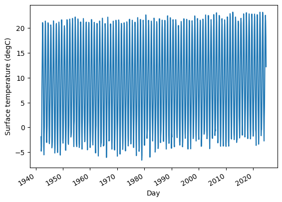
Not surprisingly, there is a strong seasonal pattern. We can use
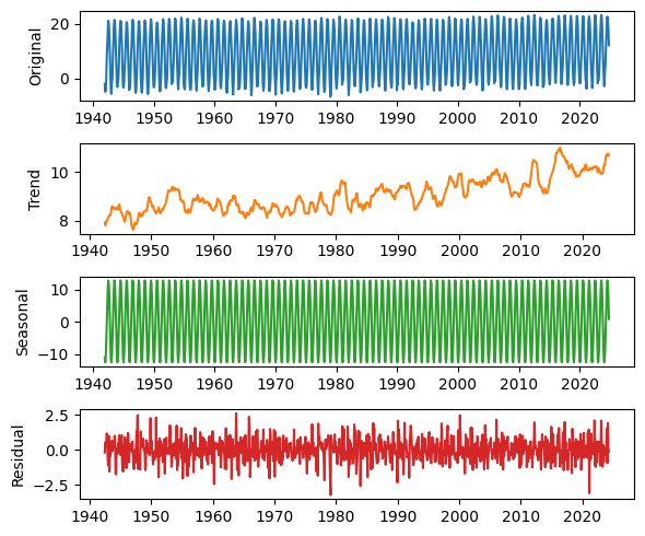
seasonal_decompose from StatsModels to identify a long-term trend, a seasonal component, and a residual.
from statsmodels.tsa.seasonal import seasonal_decompose

decomposition = seasonal_decompose(temp_series, model="additive", period=12)
We’ll use the following function to plot the results.
def plot_decomposition(original, decomposition):
    plt.figure(figsize=(6, 5))

    plt.subplot(4, 1, 1)
    plt.plot(original, label="Original", color="C0")
    plt.ylabel("Original")

    plt.subplot(4, 1, 2)
    plt.plot(decomposition.trend, label="Trend", color="C1")
    plt.ylabel("Trend")

    plt.subplot(4, 1, 3)
    plt.plot(decomposition.seasonal, label="Seasonal", color="C2")
    plt.ylabel("Seasonal")

    plt.subplot(4, 1, 4)
    plt.plot(decomposition.resid, label="Residual", color="C3")
    plt.ylabel("Residual")

    plt.tight_layout()
plot_decomposition(temp_series, decomposition)
As always, I’m grateful to Our World in Data for making datasets like this available, and now easier to use programmatically.

