Exercises

1.

We can use the methods in this chapter to estimate hazard and survival functions for the duration of a marriage. To keep things simple, we’ll consider only first marriages, and we’ll focus on divorce as the endpoint, rather than separation or death.

🔗

In the NSFG data, the cmdivorcx column contains the date of divorce for each respondent’s first marriage, if applicable, encoded in century-months. Compute the duration of marriages that have ended in divorce, and the duration, so far, of marriages that are ongoing.

🔗

For complete cases, compute the elapsed time between cmdivorcx and cmmarrhx. If both values are valid—not NaN—that means the respondent’s first marriage ended in divorce.
🔗

🔗
To identify ongoing cases, select people who have only married once and who are still married. You can use fmarno, which records the number of times each respondent has married, and rmarital, which encodes their informal marital status—the value 1 indicates that the respondent is married.
🔗

🔗

In some cases the values of these variables are only approximate, so you might find a small number of negative differences, but they should not be more than one year.

🔗

Estimate the hazard and survival functions for the duration of marriage. Plot the cumulative hazard function—when is the danger of divorce highest? Plot the survival function—what fraction of marriages end in divorce?

🔗

Listing 13.11.1. Python Code

🔗

# I suggest you use a single resampling of the data

sample = resample_cycles(resp)

🔗

2.

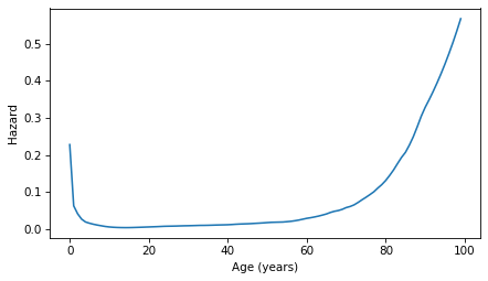
In 2012, a team of demographers at the University of Southern California estimated life expectancy for people born in Sweden in the early 1800s and 1900s. For ages from 0 to 91 years, they estimated the age-specific mortality rate, which is the fraction of people who die at a given age, out of all who survive until that age—which you might recognize as the hazard function.

🔗

I used an online graph digitizer to get the data from the figure in their paper and store it in a CSV file. Instructions for downloading the data are in the notebook for this chapter.

🔗

Data source: Beltrán-Sánchez, H., Crimmins, E. M., Finch, C. E. (2012). Early cohort mortality predicts the rate of aging in the cohort: a historical analysis. Journal of developmental origins of health and disease, 3(5), 380-386.

🔗

We can load the data like this.

🔗

Listing 13.11.2. Python Code

🔗

download(
    "https://github.com/AllenDowney/ThinkStats/raw/v3/data/mortality_rates_beltran2012.csv"
)

Listing 13.11.3. Python Code

🔗

mortality = pd.read_csv("mortality_rates_beltran2012.csv", header=[0, 1]).dropna()

The following function interpolates the data to make a hazard function with approximate mortality rates for each age from 0 to 99.

🔗

Listing 13.11.4. Python Code

🔗

from scipy.interpolate import interp1d
from empiricaldist import Hazard


def make_hazard(ages, rates):
    """Make a Hazard function by interpolating a Series.

    series: Series

    returns: Hazard
    """
    interp = interp1d(ages, rates, fill_value="extrapolate")
    xs = np.arange(0, 100)
    ys = np.exp(interp(xs))
    return Hazard(ys, xs)

Now we can make a Hazard object like this.

🔗

Listing 13.11.5. Python Code

🔗

ages = mortality["1800", "X"].values
rates = mortality["1800", "Y"].values
hazard = make_hazard(ages, rates)

Here’s what the mortality rates look like.

🔗

Listing 13.11.6. Python Code

🔗

hazard.plot()

decorate(xlabel="Age (years)", ylabel="Hazard")

Use make_surv to make a survival function based on these rates, and make_cdf to compute the corresponding CDF. Plot the results.

🔗

Then use make_pmf to make a Pmf object that represents the distribution of lifetimes, and plot it. Finally, use compute_pmf_remaining to compute the average remaining lifetime at each age from 0 to 99. Plot the result.

🔗

In the remaining lifetime curve, you should see a counterintuitive pattern—for the first few years of life, remaining lifetime increases. Because infant mortality was so high in the early 1800s, an older child was expected to live longer than a younger child. After about age 5, life expectancy returns to the pattern we expect—young people are expected to live longer than old people.

🔗

If you are interested in this topic, you might like Chapter 5 of my book, Probably Overthinking It, available from probablyoverthinking.it.

🔗

Think Stats Exploratory Data Analysis in Python

Exercises 13.11 Exercises

1.

2.