Think Stats Exploratory Data Analysis in Python

In the light bulb dataset, each value of h represents a 12-hour interval ending at hour h—which I will call “interval h”. Suppose we know that a light bulb has survived up to interval h, and we would like to know the probability that it expires during interval h. To answer this question, we can use the survival function, which indicates the fraction of bulbs that survive past interval h, and the PMF, which indicates the fraction that expire during interval h. The sum of these is the fraction of bulbs that could expire during interval h, which are said to be “at risk”. As an example, 26% of the bulbs were at risk during interval 1656.

at_risk = pmf_bulblife + surv_bulblife
at_risk[1656]

np.float64(0.25999999999999995)

And 4% of all bulbs expired during interval 1656.

pmf_bulblife[1656]

np.float64(0.04)

The hazard is the ratio of pmf_bulblife and at_risk.

hazard = pmf_bulblife / at_risk
hazard[1656]

np.float64(0.15384615384615388)

Of all bulbs that survived up to interval 1656, about 15% expired during interval 1656.

Instead of computing the hazard function ourselves, we can use empiricaldist, which provides a Hazard object that represents a hazard function, and a make_hazard method that computes it.

hazard_bulblife = surv_bulblife.make_hazard()
hazard_bulblife[1656]

np.float64(0.15384615384615397)

Here’s what the hazard function looks like for the light bulbs.

hazard_bulblife.plot()
decorate(xlabel="Light bulb duration (hours)", ylabel="Hazard")

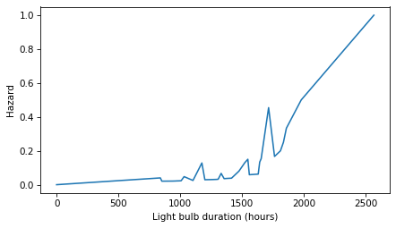
We can see that the hazard is higher in some places than others, but this way of visualizing the hazard function can be misleading, especially in parts of the range where we don’t have much data. A better alternative is to plot the cumulative hazard function, which is the cumulative sum of the hazards.

cumulative_hazard = hazard_bulblife.cumsum()
cumulative_hazard.plot()

decorate(xlabel="Light bulb duration (hours)", ylabel="Cumulative hazard")

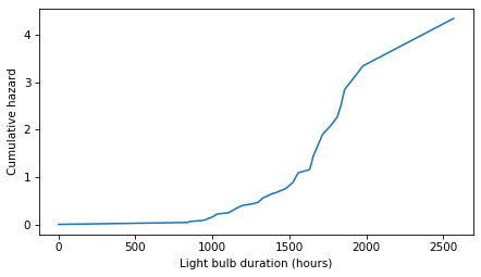
Where the probability of expiring is high, the cumulative hazard function is steep. Where the probability of expiring is low, the cumulative hazard function is flat. In this example, we can see that the hazard is highest between 1500 and 2000 hours. After that, the hazard decreases—although this outcome is based on just one unusually long-lived bulb, so it might look different in another dataset.

Now that we have the general idea of survival and hazard functions, let’s apply them to a more substantial dataset.