Autoregression

Section 12.5 Autoregression

The first idea of autoregression is that the future will be like the past. For example, in the time series we’ve looked at so far, there is a clear annual cycle. So if you are asked to make a prediction for next June, a good starting place would be last June.

🔗

To see how well that might work, let’s go back to nuclear, which contains monthly electricity production from nuclear generators, and compute differences between the same month in successive years, which are called "year-over-year" differences.

🔗

Listing 12.5.1. Python Code

🔗

diff = (nuclear - nuclear.shift(12)).dropna()
diff.plot(label="year over year differences", **actual_options)
decorate(ylabel="GWh")

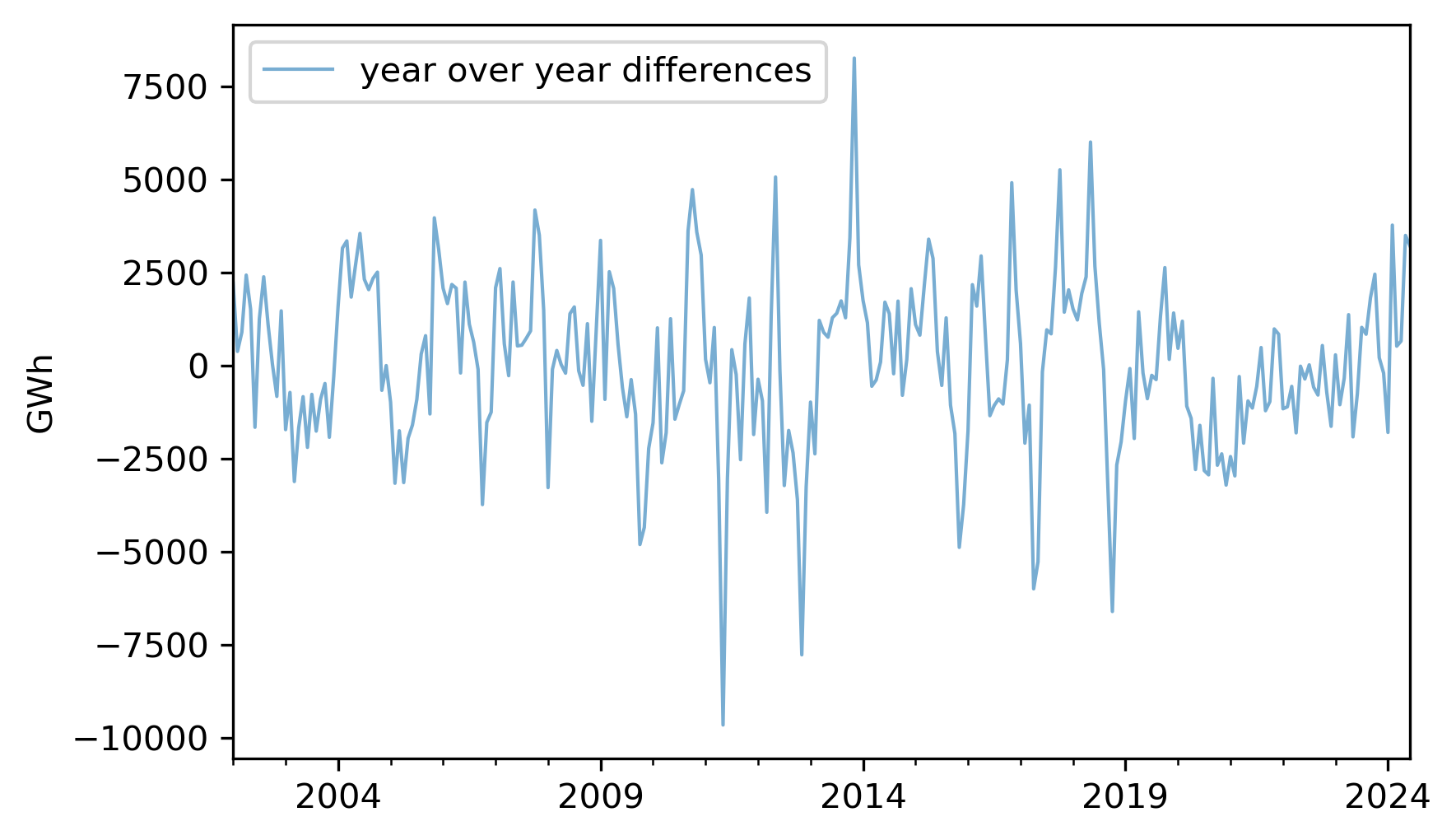
The magnitudes of these differences are substantially smaller than the magnitudes of the original series, which suggests the second idea of autoregression, which is that it might be easier to predict these differences, rather than the original values.

🔗

Toward that end, let’s see if there are correlations between successive elements in the series of differences. If so, we could use those correlations to predict future values based on previous values.

🔗

I’ll start by making a DataFrame, putting the differences in the first column and putting the same differences -- shifted by 1, 2, and 3 months -- into successive columns. These columns are named lag1, lag2, and lag3, because the series they contain have been lagged or delayed.

🔗

Listing 12.5.3. Python Code

🔗

df_ar = pd.DataFrame({"diff": diff})
for lag in [1, 2, 3]:
    df_ar[f"lag{lag}"] = diff.shift(lag)

df_ar = df_ar.dropna()

Here are the correlations between these columns.

🔗

Listing 12.5.4. Python Code

🔗

$ df_ar.corr()[["diff"]]
          diff
diff  1.000000
lag1  0.562212
lag2  0.292454
lag3  0.222228

These correlations are called lagged correlations or autocorrelations -- the prefix "auto" indicates that we’re taking the correlation of the series with itself. As a special case, the correlation between diff and lag1 is called serial correlation because it is the correlation between successive elements in the series.

🔗

These correlation are strong enough to suggest that they should help with prediction, so let’s put them into a multiple regression. The following function uses the columns from the DataFrame to make a Patsy formula with the first column as the response variable and the other columns as explanatory variables.

🔗

Listing 12.5.5. Python Code

🔗

def make_formula(df):
    """Make a Patsy formula from column names."""
    y = df.columns[0]
    xs = " + ".join(df.columns[1:])
    return f"{y} ~ {xs}"

Here are the results of a linear model that predicts the next value in a sequence based on the previous three values.

🔗

Listing 12.5.6. Python Code

🔗

formula = make_formula(df_ar)
results_ar = smf.ols(formula=formula, data=df_ar).fit()
display_summary(results_ar)

Table 12.5.7.

🔗

	coef	std err	t	P>\|t\|	[0.025	0.975]
Intercept	24.2674	114.674	0.212	0.833	-201.528	250.063
lag1	0.5847	0.061	9.528	0.000	0.464	0.706
lag2	-0.0908	0.071	-1.277	0.203	-0.231	0.049
lag3	0.1026	0.062	1.666	0.097	-0.019	0.224

Table 12.5.8.

🔗

R-squared:

0.3239

Now we can use the predict method to generate predictions for the past values in the series. Here’s what these retrodictions look like compared to the data.

🔗

Listing 12.5.9. Python Code

🔗

pred_ar = results_ar.predict(df_ar)
pred_ar.plot(label="predictions", **pred_options)
diff.plot(label="differences", **actual_options)
decorate(ylabel="GWh")

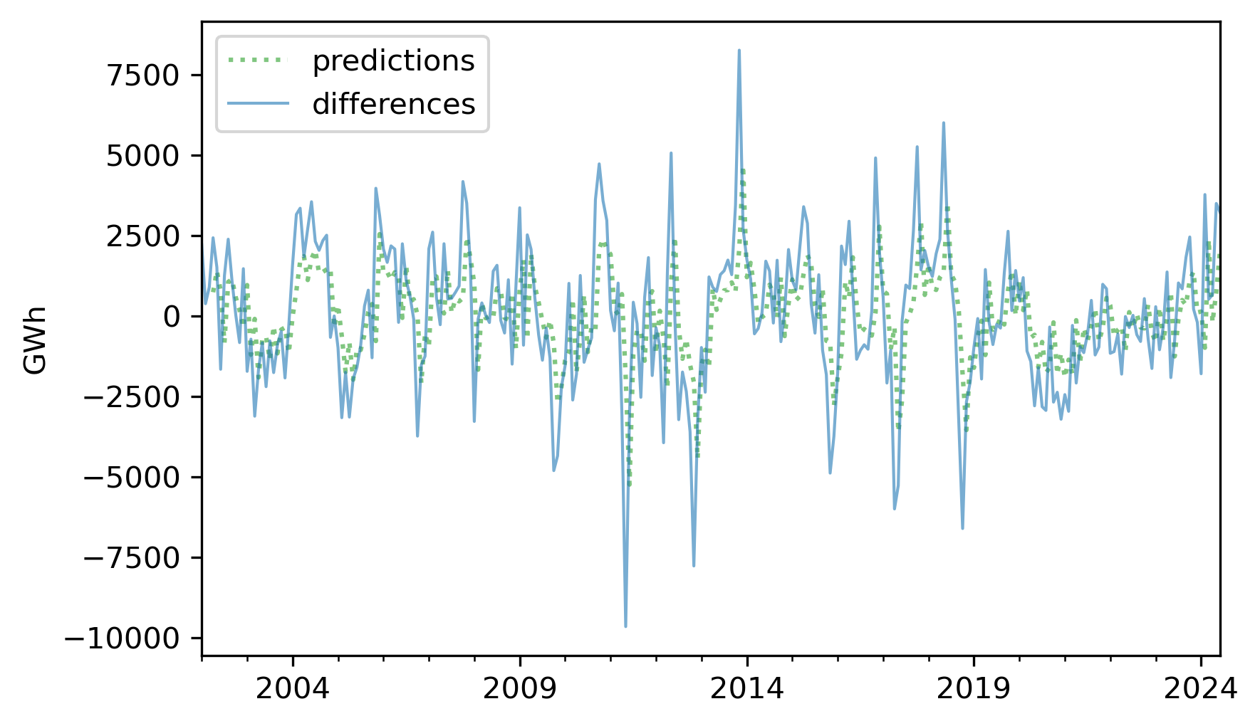
The predictions are good in some places, but the \(R^2\) value is only about 0.319, so there is room for improvement.

🔗

Listing 12.5.11. Python Code

🔗

$ resid_ar = (diff - pred_ar).dropna()
R2 = 1 - resid_ar.var() / diff.var()
R2
np.float64(0.3190252265690783)

One way to improve the predictions is to compute the residuals from this model and use another model to predict the residuals -- which is the third idea of autoregression.

🔗

Prev Top Next