Section 5.5 The Lognormal Distribution
In the previous section, we simulated pumpkin growth under the assumption that pumpkins grow 1-3 pounds per day, depending on the weather. Instead, let’s suppose their growth is proportional to their current weight, so big pumpkins gain more weight per day than small pumpkins — which is probably more realistic.
The following function simulates this kind of proportional growth, where a pumpkin gains 3% of its weight if the weather is bad, 5% if the weather is fair, and 7% if the weather is good. We’ll assume that the weather is bad, fair, or good on any given day with equal probability.
def simulate_proportionate_growth(n):
    choices = [1.03, 1.05, 1.07]
    gains = np.random.choice(choices, n)
    return gains.prod()
If a pumpkin gains 3% of its weight, the final weight is the product of the initial weight and the factor 1.03. So we can compute the weight after 100 days by choosing random factors and multiplying them together. We’ll call this function 1001 times to simulate 1001 pumpkins and save their weights. The average weight is about 131 pounds; the standard deviation is about 21 pounds. So the pumpkins in this model are smaller but more variable than in the previous model.
$ sim_weights = [simulate_proportionate_growth(100) for i in range(1001)]
np.mean(sim_weights), np.std(sim_weights)
(np.float64(130.80183363824722), np.float64(20.956047434921466))
We can show mathematically that these weights follow a lognormal distribution, which means that the logarithms of the weights follow a normal distribution. To check, we’ll compute the logs of the weights and their mean and standard deviation. We could use logarithms with any base, but I’ll use base 10 because it makes the results easier to interpret.
$ log_sim_weights = np.log10(sim_weights)
m, s = np.mean(log_sim_weights), np.std(log_sim_weights)
m, s
(np.float64(2.1111299372609933), np.float64(0.06898607064749827))
Now let’s compare the distribution of the logarithms to a normal distribution with the same mean and standard deviation.
cdf_model = make_normal_model(log_sim_weights)
cdf_log_sim_weights = Cdf.from_seq(log_sim_weights, name="simulation")

two_cdf_plots(
    cdf_model, cdf_log_sim_weights, xlabel="Pumpkin weight (log10 pounds)"
)
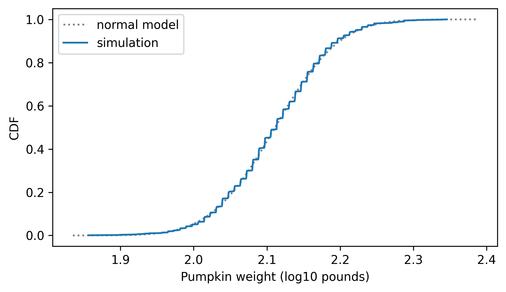
The model fits the simulation result very well, which is what we expected.
If people are like pumpkins, where the change in weight from year to year is proportionate to their current weight, we might expect the distribution of adult weights to follow a lognormal distribution. Let’s find out.
The National Center for Chronic Disease Prevention and Health Promotion conducts an annual survey as part of the Behavioral Risk Factor Surveillance System (BRFSS). In 2008, they interviewed 414,509 respondents and asked about their demographics, health, and health risks. Among the data they collected are the weights of 398,484 respondents.
The
thinkstats module provides a function that reads BRFSS data and returns a Pandas DataFrame. Adult weights in kilograms are recorded in the wtkg2 column. The mean is about 79 kg.
download("https://github.com/AllenDowney/ThinkStats/raw/v3/data/CDBRFS08.ASC.gz")
from thinkstats import read_brfss

brfss = read_brfss()
Adult weights in kilograms are recorded in the
wtkg2 column.
$ adult_weights = brfss["wtkg2"].dropna()
m, s = np.mean(adult_weights), np.std(adult_weights)
m, s
(np.float64(78.9924529968581), np.float64(19.546132387397257))
The mean is about 79 kg. Before we compute logarithms, let’s see if the weights follow a normal distribution.
cdf_model = make_normal_model(adult_weights)
cdf_adult_weights = Cdf.from_seq(adult_weights, name="adult weight")

two_cdf_plots(cdf_model, cdf_adult_weights, xlabel="Adult weight (kilograms)")
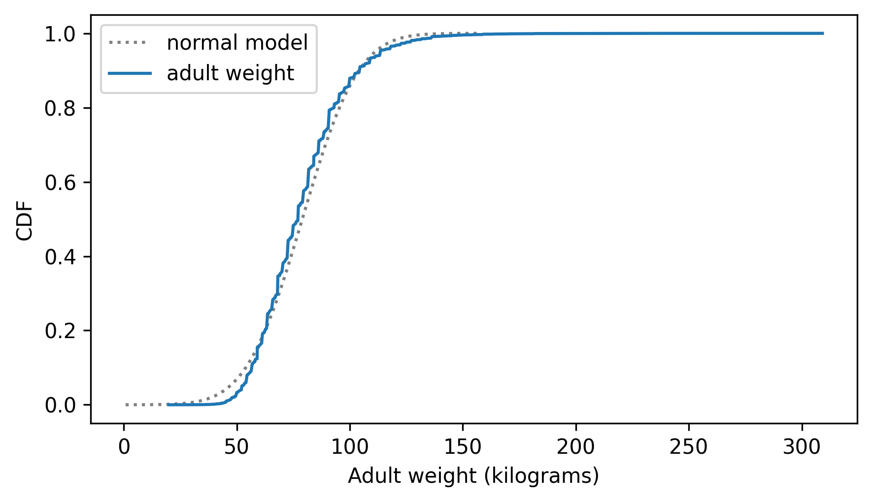
The normal distribution might be a good enough model for this data, for some purposes — but let’s see if we can do better. Here’s the distribution of the log-transformed weights and a normal model with the same mean and standard deviation.
log_adult_weights = np.log10(adult_weights)
cdf_model = make_normal_model(log_adult_weights)

cdf_log_adult_weights = Cdf.from_seq(log_adult_weights, name="log adult weight")
two_cdf_plots(cdf_model, cdf_log_adult_weights, xlabel="Adult weight (log10 kg)")
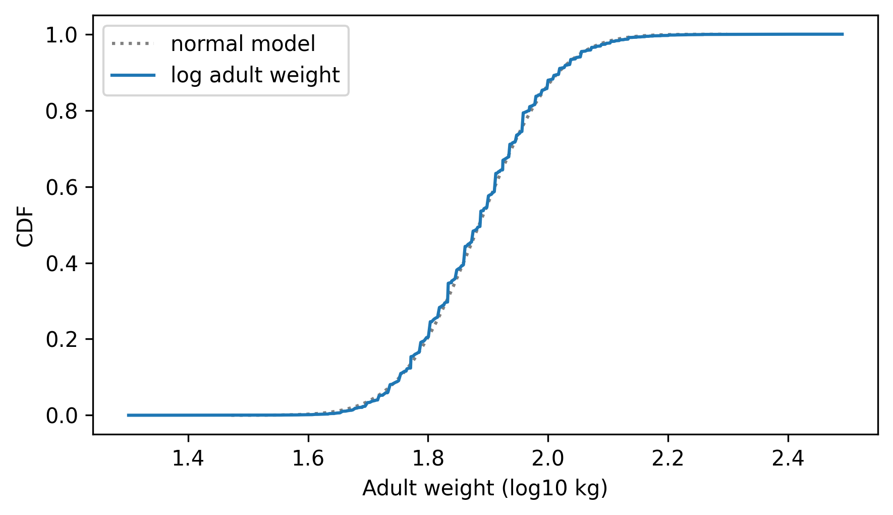
The normal model fits the logarithms better than it fits the weights themselves, which suggests that proportional growth is a better model of weight gain than additive growth.

