Section 14.8 Correlation Test
In Chapter 9 we used a permutation test for the correlation between birth weight and mother’s age, and found that it is statistically significant, with p-value less than 0.001.
Now we can do the same thing analytically. The method is based on this mathematical result: If we generate two samples with size
n from normal distributions, compute Pearson’s correlation, r, and then transform the correlation with this function:
def transform_correlation(r, n):
    return r * np.sqrt((n - 2) / (1 - r**2))
The transformed correlations follow a \(t\) distribution with parameter
n-2. To see what that looks like, we’ll use the following function to generate uncorrelated samples from a standard normal distribution.
def generate_data(n):
    """Uncorrelated sequences from a standard normal."""
    xs = np.random.normal(0, 1, n)
    ys = np.random.normal(0, 1, n)
    return xs, ys
And the following function to compute their correlation.
def correlation(data):
    xs, ys = data
    return np.corrcoef(xs, ys)[0, 1]
The following loop generates many pairs of samples, computes their correlation, and puts the results in a list.
n = 100
rs = [correlation(generate_data(n)) for i in range(1001)]
Next we’ll compute the transformed correlations.
ts = transform_correlation(np.array(rs), n)
To check whether these
ts follow a \(t\) distribution, we’ll use the following function, which makes an object that represents the CDF of a \(t\) distribution.
from scipy.stats import t as student_t


def make_student_cdf(df):
    """Computes the CDF of a Student t distribution."""
    ts = np.linspace(-3, 3, 101)
    ps = student_t.cdf(ts, df=df)
    return Cdf(ps, ts)
The parameter of the \(t\) distribution is called
df, which stands for “degrees of freedom”. The following figure shows the CDF of a \(t\) distribution with parameter n-2 along with the empirical CDF of the transformed correlations.
make_student_cdf(df=n - 2).plot(**model_options)

cdf_ts = Cdf.from_seq(ts)
cdf_ts.plot(label="random normals")

decorate(xlabel="Transformed correlation", ylabel="CDF")
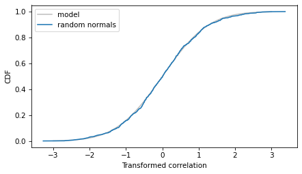
This shows that if we draw uncorrelated samples from normal distributions, their transformed correlations follow a \(t\) distribution.
If we draw samples from other distributions, their transformed correlations don’t follow a \(t\) distribution exactly, but they converge to a \(t\) distribution as the sample size increases. Let’s see if this applies to the correlation of maternal age and birth weight. From the
DataFrame of live births, we’ll select the rows with valid data.
$ valid = live.dropna(subset=["agepreg", "totalwgt_lb"])
n = len(valid)
n
9038
The actual correlation is about 0.07.
$ data = valid["agepreg"].values, valid["totalwgt_lb"].values
r_actual = correlation(data)
r_actual
np.float64(0.0688339703541091)
def permute(data):
    """Shuffle the x values."""
    xs, ys = data
    new_xs = xs.copy()
    np.random.shuffle(new_xs)
    return new_xs, ys
If we generate many permutations and compute their correlations, the result is a sample from the distribution of correlations under the null hypothesis.
permuted_corrs = [correlation(permute(data)) for i in range(1001)]
And we can compute the transformed correlations like this.
ts = transform_correlation(np.array(permuted_corrs), n)
The following figure shows the empirical CDF of the
ts along with the CDF of the \(t\) distribution with parameter n-2.
make_student_cdf(n - 2).plot(**model_options)
Cdf.from_seq(ts).plot(label="permuted data")

decorate(xlabel="Transformed correlation", ylabel="CDF")
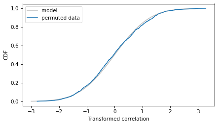
The model fits the empirical distribution well, which means we can use it to compute a p-value for the observed correlation. First we’ll transform the observed correlation.
t_actual = transform_correlation(r_actual, n)
Now we can use the CDF of the \(t\) distribution to compute the probability of a value as large as
t_actual under the null hypothesis.
$ right = 1 - student_t.cdf(t_actual, df=n - 2)
right
np.float64(2.8614777214386322e-11)
We can also compute the probability of a value as negative as
-t_actual.
$ left = student_t.cdf(-t_actual, df=n - 2)
left
np.float64(2.8614735536574038e-11)
The sum of the two is the probability of a correlation as big as
r_actual, positive or negative.
$ left + right
np.float64(5.722951275096036e-11)
SciPy provides a function that does the same calculation and returns the p-value of the observed correlation.
$ from scipy.stats import pearsonr

corr, p_value = pearsonr(*data)
p_value
np.float64(5.722947107314364e-11)
The results are nearly the same.
Based on the resampling results, we concluded that the p-value was less than 0.001, but we could not say how much less without running a very large number of resamplings. With analytic methods, we can compute small p-values quickly.
However, in practice it might not matter. Generally, if a p-value is smaller than 0.001, we can conclude that the observed effect is unlikely to be due to chance. It is not usually important to know precisely how unlikely.

