Central Limit Theorem

Section 14.5 Central Limit Theorem

As we saw in the previous sections, if we add values drawn from normal distributions, the distribution of the sum is normal. Most other distributions don’t have this property—for example, if we add values drawn from an exponential distribution, the distribution of the sum is not exponential.

🔗

But for many distributions, if we generate n values and add them up, the distribution of the sum converges to normal as n increases. More specifically, if the distribution of the values has mean m and variance s2 the distribution of the sum converges to a normal distribution with mean n * m and variance n * s2.

🔗

That conclusion is the Central Limit Theorem (CLT). It is one of the most useful tools for statistical analysis, but it comes with caveats:

🔗

The values have to come from the same distribution (although this requirement can be relaxed).
🔗

🔗
The values have to be drawn independently. If they are correlated, the CLT doesn’t apply (although it can still work if the correlation is not too strong).
🔗

🔗
The values have to be drawn from a distribution with finite mean and variance. So the CLT doesn’t apply to some long-tailed distributions.
🔗

🔗

The Central Limit Theorem explains the prevalence of normal distributions in the natural world. Many characteristics of living things are affected by genetic and environmental factors whose effect is additive. The characteristics we measure are the sum of a large number of small effects, so their distribution tends to be normal.

🔗

To see how the Central Limit Theorem works, and when it doesn’t, let’s try some experiments, starting with an exponential distribution. The following loop generates samples from an exponential distribution, adds them up, and makes a dictionary that maps from each sample size, n, to a list of 1001 sums.

🔗

Listing 14.5.1. Python Code

🔗

np.random.seed(17)

Listing 14.5.2. Python Code

🔗

lam = 1
df_sample_expo = pd.DataFrame()
for n in [1, 10, 100]:
    df_sample_expo[n] = [np.sum(np.random.exponential(lam, n)) for _ in range(1001)]

Here are the averages for each list of sums.

🔗

Listing 14.5.3. Python Code

🔗

$ df_sample_expo.mean()
1        0.989885
10       9.825744
100    100.022555
dtype: float64

The average value from this distribution is 1, so if we add up 10 values, the average of the sum is close to 10, and if we add up 100 values the average of the sum is close to 100.

🔗

This function takes the DataFrame we just made and makes a normal probability plot for each list of sums.

🔗

Listing 14.5.4. Python Code

🔗

def normal_plot_samples(df_sample, ylabel=""):
    """Normal probability plots for samples of sums."""
    plt.figure(figsize=(6.8, 2.6))
    for i, n in enumerate(df_sample):
        plt.subplot(1, 3, i + 1)
        normal_probability_plot(df_sample[n])
        decorate(
            title="n=%d" % n,
            xticks=[],
            yticks=[],
            xlabel="Standard normal",
            ylabel=ylabel,
        )

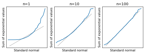
The following figure shows normal probability plots for the three lists of sums (the definition of normal_plot_samples is in the notebook for this chapter).

🔗

Listing 14.5.5. Python Code

🔗

normal_plot_samples(df_sample_expo, ylabel="Sum of exponential values")

When n=1, the distribution of the sum is exponential, so the normal probability plot is not a straight line. But with n=10 the distribution of the sum is approximately normal, and with n=100 it is almost indistinguishable from normal.

🔗

For distributions that are less skewed than an exponential, the distribution of the sum converges to normal more quickly—that is, for smaller values of n. For distributions that are more skewed, it takes longer. As an example, let’s look at sums of values from a lognormal distribution.

🔗

Listing 14.5.7. Python Code

🔗

mu, sigma = 3.0, 1.0
df_sample_lognormal = pd.DataFrame()
for n in [1, 10, 100]:
    df_sample_lognormal[n] = [
        np.sum(np.random.lognormal(mu, sigma, n)) for _ in range(1001)
    ]

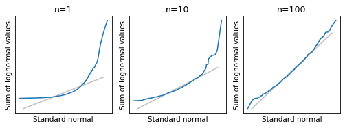
Here are the normal probability plots for the same range of sample sizes.

🔗

Listing 14.5.8. Python Code

🔗

normal_plot_samples(df_sample_lognormal, ylabel="Sum of lognormal values")

When n=1, a normal model does not fit the distribution, and it is not much better with n=10. Even with n=100, the tails of the distribution clearly deviate from the model.

🔗

The mean and variance of the lognormal distribution are finite, so the distribution of the sum converges to normal eventually. But for some highly skewed distributions, it might not converge at any practical sample size. And in some cases, it doesn’t happen at all.

🔗

Prev Top Next