Section 8.4 Sampling Distributions
So far we’ve been working with simulated data, assuming that penguin weights are drawn from a normal distribution with known parameters. Now let’s see what happens with real data.
Between 2007 and 2010, researchers at Palmer Station in Antarctica measured and weighed 342 penguins from local populations. The data they collected is freely available -- instructions for downloading it are in the notebook for this chapter.
The following cell downloads the data from a repository created by Allison Horst.
Horst AM, Hill AP, Gorman KB (2020). palmerpenguins: Palmer Archipelago (Antarctica) penguin data. R package version 0.1.0. https://allisonhorst.github.io/palmerpenguins/. doi: 10.5281/zenodo.3960218.
The data was collected as part of the research that led to this paper: Gorman KB, Williams TD, Fraser WR (2014). Ecological sexual dimorphism and environmental variability within a community of Antarctic penguins (genus Pygoscelis). PLoS ONE 9(3):e90081. https://doi.org/10.1371/journal.pone.0090081
download(
    "https://raw.githubusercontent.com/allisonhorst/palmerpenguins/c19a904462482430170bfe2c718775ddb7dbb885/inst/extdata/penguins_raw.csv"
)
We can use Pandas to read the data.
$ penguins = pd.read_csv("penguins_raw.csv").dropna(subset=["Body Mass (g)"])
penguins.shape
(342, 17)
The dataset includes three penguin species.
$ penguins["Species"].value_counts()
Species
Adelie Penguin (Pygoscelis adeliae)          151
Gentoo penguin (Pygoscelis papua)            123
Chinstrap penguin (Pygoscelis antarctica)     68
Name: count, dtype: int64
For the first example we’ll select just the Chinstrap penguins.
chinstrap = penguins.query('Species.str.startswith("Chinstrap")')
We’ll use this function to plot estimated PDFs.
def plot_kde(sample, name="estimated density", **options):
    kde = gaussian_kde(sample)
    m, s = np.mean(sample), np.std(sample)
    plt.axvline(m, color="gray", ls=":")

    domain = m - 4 * s, m + 4 * s
    pdf = Pdf(kde, domain, name)
    pdf.plot(**options)
Here’s the distribution of chinstrap penguin weights in kilograms. The vertical dotted line shows the sample mean.
weights = chinstrap["Body Mass (g)"] / 1000
plot_kde(weights, "weights")
decorate(xlabel="Penguin weight (kg)", ylabel="Density")
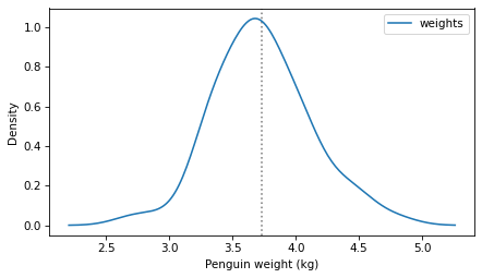
The sample mean is about 3.7 kg.
$ sample_mean = np.mean(weights)
sample_mean
np.float64(3.733088235294118)
If you are asked to estimate the population mean, 3.7 kg is a reasonable choice -- but how precise is that estimate?
One way to answer that question is to compute the sampling distribution of the mean, which shows how much the estimated mean varies from one sample to another. If we knew the actual mean and standard deviation in the population, we could model the sampling process and compute the sampling distribution. But if we knew the actual population mean, we wouldn’t have to estimate it!
Fortunately, there’s a simple way to approximate the sampling distribution, called resampling. The core idea is to use the sample to make a model of the population, then use the model to simulate the sampling process.
More specifically, we’ll use parametric resampling, which means we’ll use the sample to estimate the parameters of the population and then use a theoretical distribution to generate new samples.
The following function implements this process with a normal distribution. Notice that the new samples are the same size as the original.
def resample(sample):
    # Generate a sample from a normal distribution
    m, s = np.mean(sample), np.std(sample)
    return np.random.normal(m, s, len(sample))
This loop uses
resample to generate many samples and compute the mean of each one.
sample_means = [np.mean(resample(weights)) for i in range(1001)]
The following figure shows the distribution of these sample means.
plot_kde(sample_means, "sample means")
decorate(xlabel="Sample mean of weight (kg)", ylabel="Density")
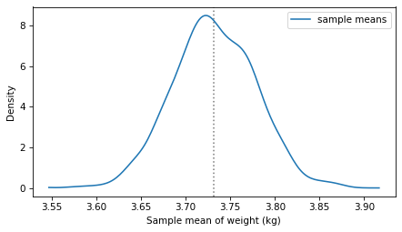
This result approximates the sampling distribution of the sample mean. It shows how much we expect the sample mean to vary if we collect many samples of the same size -- assuming that our model of the population is accurate.
Informally, we can see that the sample mean could be as low as 3.55, if we collected another sample with the same size, or as high as 3.9.

