Section 13.5 Estimating Hazard Functions
In the light bulb example, we know the life spans for all 50 bulbs, so we can compute the survival function directly—and we can use the survival function to compute the hazard function.
In the marriage example, we know the age at first marriage for some respondents, the ones who had been married before they were interviewed. But for respondents who had never married, we don’t know at what age they would marry in the future—or if they will.
This kind of missing data is said to be censored. That term might seem odd, because censored information is usually hidden deliberately, but in this case it is hidden just because we don’t know the future.
However, we have partial information we can work with: if someone is unmarried when they are surveyed, we know that the age when they get married (if they do) must be greater than their current age.
We can use this partial information to estimate the hazard function; then we can use the hazard function to compute the survival function. This process is called Kaplan-Meier estimation.
To demonstrate, I’ll select just one cohort from the resampled data.
resp60 = sample.query("cohort == 1960")
For respondents who were married when they were surveyed, we’ll select their age at first marriage. There are 9921 of them, which we’ll call “complete” cases.
complete = resp60.query("evrmarry == 1")["agemarr"]
complete.count()
np.int64(9921)
For respondents who had not married, we’ll select their age when they were surveyed. There are 5468 of them, which we’ll call the “ongoing” cases.
ongoing = resp60.query("evrmarry == 0")["age"]
ongoing.count()
np.int64(5468)
Now, to estimate the hazard function, we’ll compute the total number of cases that were “at risk” at each age, including everyone who was unmarried up to that age. It will be convenient to make a
FreqTab object that counts the number of complete and ongoing cases at each age.
from empiricaldist import FreqTab

ft_complete = FreqTab.from_seq(complete)
ft_ongoing = FreqTab.from_seq(ongoing)
As an example, there are 58 respondents who reported that they were married for the first time at age 25.
ft_complete[25]
np.int64(58)
And another 5 respondents who were surveyed at age 25 and reported that they had never married.
ft_ongoing[25]
np.int64(5)
From these
FreqTab objects, we can compute unnormalized Surv objects that contain the number of complete and ongoing cases that exceed each age.
surv_complete = ft_complete.make_surv()
surv_ongoing = ft_ongoing.make_surv()
For example, there are 2848 people who reported getting married after age 25.
surv_complete[25]
np.int64(2848)
And 2273 people surveyed after age 25 who had never married.
surv_ongoing[25]
np.int64(2273)
The sum of the four numbers we just computed is the number of respondents who were at risk—that is, people who could have married at age 25. The term “at risk” is a legacy of survival analysis in medicine, where it often refers to risk of disease or death. It might seem incongruent in the context of marriage, which is generally considered a positive milestone. That said, here’s how we compute it.
at_risk = ft_complete[25] + ft_ongoing[25] + surv_complete[25] + surv_ongoing[25]
at_risk
np.int64(5184)
Of those, the number who actually married at age 25 is
ft_complete[25]. So we can compute the hazard function at age 25 like this.
hazard = ft_complete[25] / at_risk
hazard
np.float64(0.011188271604938271)
That’s how we can compute the hazard function at a single age. Now let’s compute the whole function, for all ages. We’ll use the
union method of the Index class to compute a Pandas Index that contains all of the ages from ft_complete and ft_ongoing, in order.
ts = pd.Index.union(ft_complete.index, ft_ongoing.index)
Now we can compute the number of people at risk at every age, by looking up the ages in
ts in each of the FreqTab and Surv objects.
at_risk = ft_complete(ts) + ft_ongoing(ts) + surv_complete(ts) + surv_ongoing(ts)
Finally, we can compute the hazard function at each age, and put the results into a
Hazard object.
from empiricaldist import Hazard

hs = ft_complete(ts) / at_risk
hazard = Hazard(hs, ts)
Here’s what the cumulative hazard function looks like.
hazard.cumsum().plot()

decorate(xlabel="Age", ylabel="Cumulative hazard")
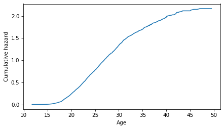
It is steepest between ages 20 and 30, which means that an unmarried person is at the greatest “risk” of getting married at these ages. After that, the cumulative hazard levels off, which means that the hazard gradually decreases.

