The Exponential Distribution

Section 5.3 The Exponential Distribution

In the previous section, we simulated a simple model of a hockey game where a goal has the same probability of being scored during any second of the game. Under the same model, it turns out, the time until the first goal follows an exponential distribution.

🔗

To demonstrate, let’s assume again that the teams score a total of 6 goals, on average, and compute the probability of a goal during each second.

🔗

Listing 5.3.1. Python Code

🔗

$ n = 3600
m = 6
p = m / 3600
p
0.0016666666666666668

The following function simulates n seconds and uses argmax to find the time of the first goal. This works because the result from flip is a sequence of 1s and 0s, so the maximum is almost always 1. If there is at least one goal in the sequence, argmax returns the index of the first. If there are no goals, it returns 0, but that happens seldom enough that we’ll ignore it.

🔗

Listing 5.3.2. Python Code

🔗

def simulate_first_goal(n, p):
    return flip(n, p).argmax()

We’ll use simulate_first_goal to simulate 1001 games and make a list of the times until the first goal. The average time until the first goal is close to 600 seconds, or 10 minutes. And that makes sense — if we expect 6 goals per sixty-minute game, we expect one goal every 10 minutes, on average.

🔗

Listing 5.3.3. Python Code

🔗

np.random.seed(3)

Listing 5.3.4. Python Code

🔗

$ first_goal_times = [simulate_first_goal(n, p) for i in range(1001)]
mean = np.mean(first_goal_times)
mean
np.float64(597.7902097902098)

When n is large and p is small, we can show mathematically that the expected time until the first goal follows an exponential distribution. The CDF of the exponential distribution is easy to compute.

🔗

Listing 5.3.5. Python Code

🔗

def exponential_cdf(x, lam):
    """Compute the exponential CDF.

    x: float or sequence of floats
    lam: rate parameter

    returns: float or NumPy array of cumulative probability
    """
    return 1 - np.exp(-lam * x)

The value of lam is the average number of events per unit of time — in this example it is goals per second. We can use the mean of the simulated results to compute lam.

🔗

Listing 5.3.6. Python Code

🔗

$ lam = 1 / mean
lam
np.float64(0.0016728276636563566)

If we call this function with a range of time values, we can approximate the distribution of first goal times. The NumPy function linspace creates an array of equally-spaced values; in this example, it computes 201 values from 0 to 3600, including both.

🔗

Listing 5.3.7. Python Code

🔗

from empiricaldist import Cdf

ts = np.linspace(0, 3600, 201)
ps = exponential_cdf(ts, lam)
cdf_expo = Cdf(ps, ts, name="exponential model")

The following figure compares the simulation results to the exponential distribution we just computed.

🔗

Listing 5.3.8. Python Code

🔗

cdf_sim = Cdf.from_seq(first_goal_times, name="simulation")

cdf_expo.plot(ls=":", color="gray")
cdf_sim.plot()

decorate(xlabel="Time of first goal (seconds)", ylabel="CDF")

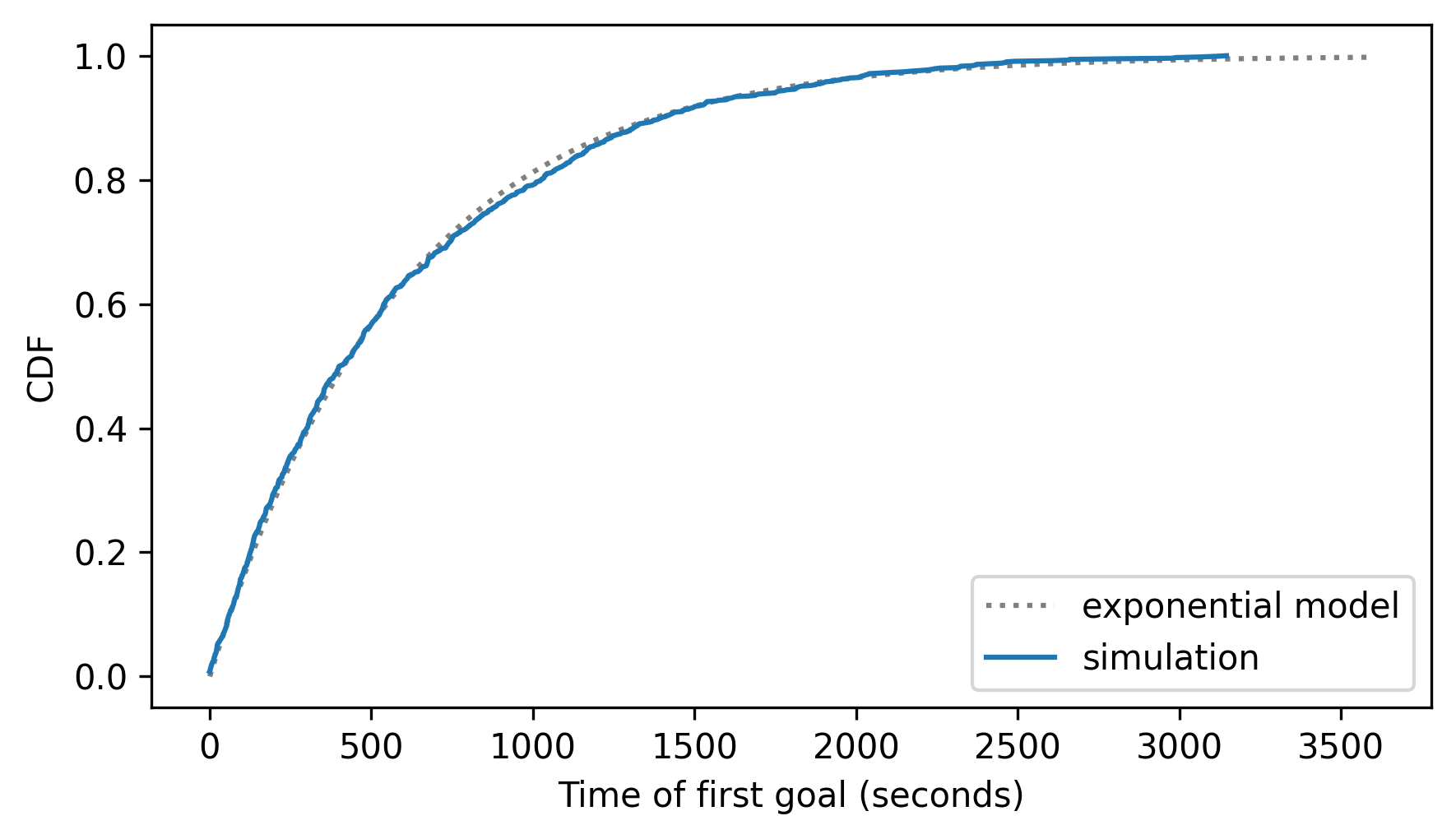
The exponential model fits the results from the simulation very well — but a stronger test is to see how it does with real data.

🔗

The following loop reads the results for all games, gets the time of the first goal, and stores the result in a list. If no goals were scored, it adds nan to the list.

🔗

Listing 5.3.10. Python Code

🔗

filename = "nhl_2023_2024.hdf"

with pd.HDFStore(filename, "r") as store:
    keys = store.keys()

Listing 5.3.11. Python Code

🔗

firsts = []

for key in keys:
    times = pd.read_hdf(filename, key=key)
    if len(times) > 0:
        firsts.append(times[0])
    else:
        firsts.append(np.nan)

To estimate the goal-scoring rate, we can use nanmean, which computes the mean of the times, ignoring nan values.

🔗

Listing 5.3.12. Python Code

🔗

$ lam = 1 / np.nanmean(firsts)
lam
np.float64(0.0015121567467720825)

Now we can compute the CDF of an exponential distribution with the same goal-scoring rate as the data, and compare it to the CDF of the data, using the dropna=False argument to include nan values at the end.

🔗

Listing 5.3.13. Python Code

🔗

ps = exponential_cdf(ts, lam)
cdf_expo = Cdf(ps, ts, name="exponential model")

Listing 5.3.14. Python Code

🔗

$ cdf_firsts = Cdf.from_seq(firsts, name="data", dropna=False)
cdf_firsts.tail()
3286.0    0.996951
3581.0    0.997713
NaN       1.000000
Name: data, dtype: float64

Listing 5.3.15. Python Code

🔗

cdf_expo.plot(ls=":", color="gray")
cdf_firsts.plot()

decorate(xlabel="Time of first goal (seconds)", ylabel="CDF")

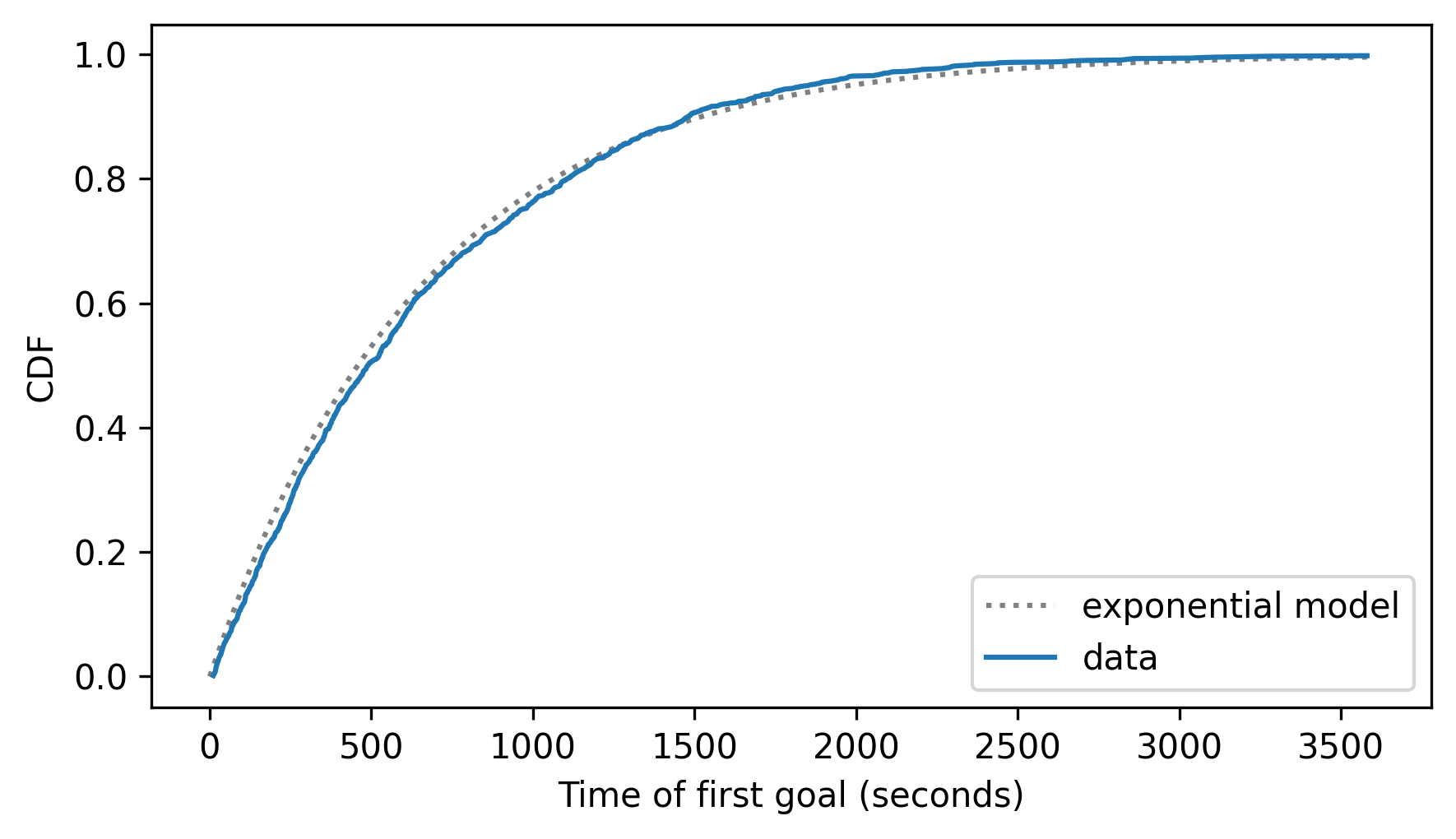
The data deviate from the model in some places — it looks like there are fewer goals in the first 1000 seconds than the model predicts. But still, the model fits the data well.

🔗

The underlying assumption of these models — the Poisson model of goals and the exponential model of times — is that a goal is equally likely during any second of a game. If you ask a hockey fan whether that’s true, they would say no, and they would be right — the real world violates assumptions like these in many ways. Nevertheless, theoretical distributions often fit real data remarkably well.

🔗

Prev Top Next