ARIMA

Section 12.8 ARIMA

StatsModel provides a library called tsa, which stands for "time series analysis" -- it includes a function called ARIMA that fits ARIMA models and generates forecasts.

🔗

To fit the SARIMA model we developed in the previous sections, we’ll call this function with two tuples as arguments: order and seasonal_order. Here are the values in order that correspond to the model we used in the previous sections.

🔗

Listing 12.8.1. Python Code

🔗

order = ([1, 2, 3], 0, [1, 6])

The values in order indicate:

🔗

Which lags should be included in the AR model -- in this example it’s the first three.
🔗

🔗
How many times it should compute differences between successive elements -- in this example it’s 0 because we computed a seasonal difference instead, and we’ll get to that in a minute.
🔗

🔗
Which lags should be included in the MA model -- in this example it’s the first and sixth.
🔗

🔗

Now here are the values in seasonal_order.

🔗

Listing 12.8.2. Python Code

🔗

seasonal_order = (0, 1, 0, 12)

The first and third elements are 0, which means that this model does not include seasonal AR or seasonal MA. The second element is 1, which means it computes seasonal differences -- and the last element is the seasonal period.

🔗

Here’s how we use ARIMA to make and fit this model.

🔗

Listing 12.8.3. Python Code

🔗

import statsmodels.tsa.api as tsa

model = tsa.ARIMA(nuclear, order=order, seasonal_order=seasonal_order)
results_arima = model.fit()
display_summary(results_arima)

Table 12.8.4.

🔗

	coef	std err	z	P>\|z\|	[0.025	0.975]
ar.L1	0.0458	0.379	0.121	0.904	-0.697	0.788
ar.L2	-0.0035	0.116	-0.030	0.976	-0.230	0.223
ar.L3	0.0375	0.049	0.769	0.442	-0.058	0.133
ma.L1	0.2154	0.382	0.564	0.573	-0.533	0.964
ma.L6	-0.0672	0.019	-3.500	0.000	-0.105	-0.030
sigma2	3.473e+06	1.9e-07	1.83e+13	0.000	3.47e+06	3.47e+06

The results include estimated coefficients for the three lags in the AR model, the two lags in the MA model, and sigma2, which is the variance of the residuals.

🔗

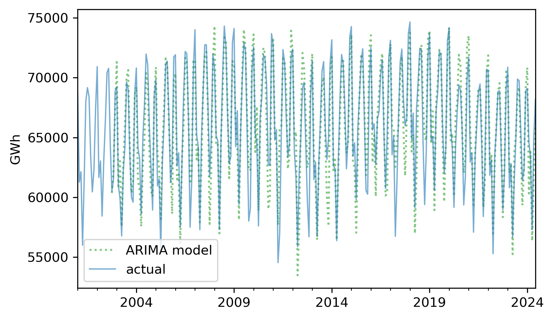
From results_arima we can extract fittedvalues, which contains the retrodictions. For the same reason there were missing values at the beginning of the retrodictions we computed, there are incorrect values at the beginning of fittedvalues, which we’ll drop.

🔗

Listing 12.8.5. Python Code

🔗

fittedvalues = results_arima.fittedvalues[n_missing:]

The fitted values are similar to the ones we computed, but not exactly the same -- probably because ARIMA handles the initial conditions differently.

🔗

Listing 12.8.6. Python Code

🔗

fittedvalues.plot(label="ARIMA model", **pred_options)
nuclear.plot(label="actual", **actual_options)
decorate(ylabel="GWh")

The \(R^2\) value is also similar but not precisely the same.

🔗

Listing 12.8.8. Python Code

🔗

$ resid = fittedvalues - nuclear
R2 = 1 - resid.var() / nuclear.var()
R2
np.float64(0.8262717330822065)

The ARIMA function makes it easy to experiment with different versions of the model.

🔗

As an exercise, try out different values in order and seasonal_order and see if you can find a model with higher \(R^2\text{.}\)

🔗

Prev Top Next