Section 12.4 Multiplicative Model
The additive model we used in the previous section assumes that the time series is the sum of a long-term trend, a seasonal component, and a residual -- which implies that the magnitude of the seasonal component and the residuals does not vary over time.
As an example that violates this assumption, let’s look at small-scale solar electricity production since 2014.
solar = elec["United States : small-scale solar photovoltaic"].dropna()
solar.plot(label="solar", **actual_options)
decorate(ylabel="GWh")
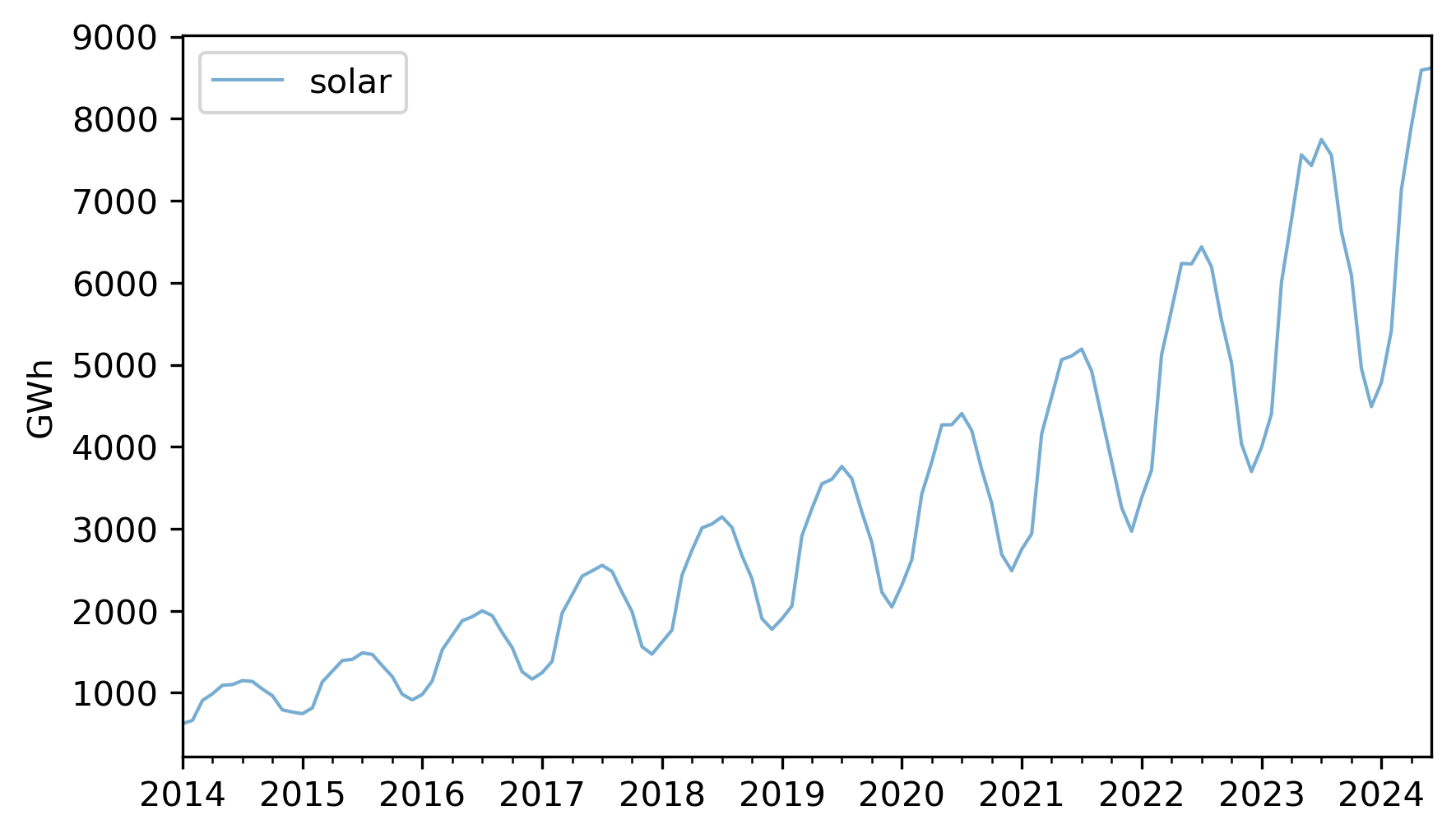
Over this interval, total production has increased several times over. And it’s clear that the magnitude of seasonal variation has increased as well.
If we suppose that the magnitudes of seasonal and random variation are proportional to the magnitude of the trend, that suggests an alternative to the additive model in which the time series is the product of the three components.
To try out this multiplicative model, we’ll split this series into training and test sets.
training, test = split_series(solar)
decomposition = seasonal_decompose(training, model="multiplicative", period=12)
Here’s what the results look like.
plot_decomposition(training, decomposition)
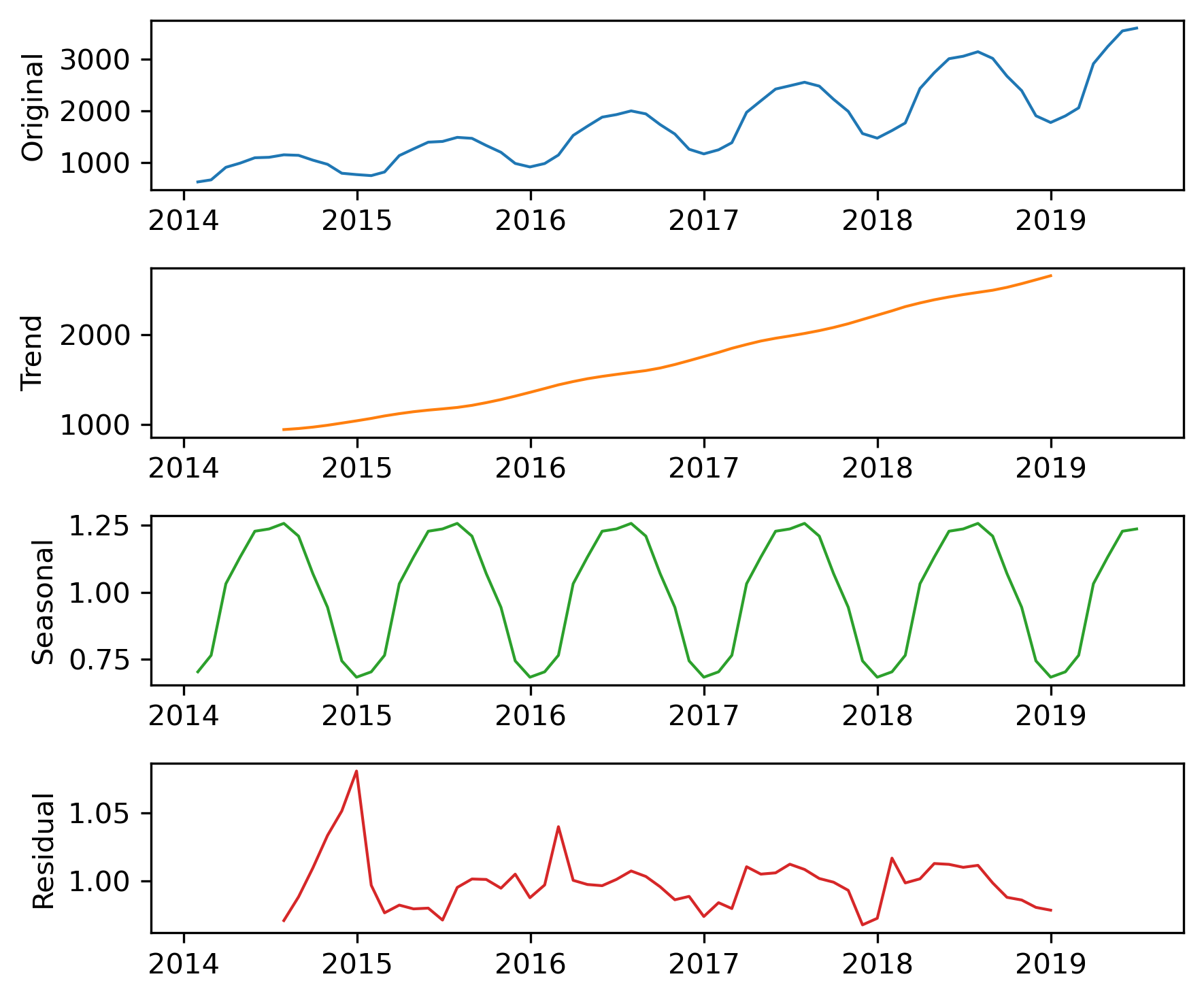
Now the seasonal and residual components are multiplicative factors. So, it looks like the seasonal component varies from about 25% below the trend to 25% above. And the residual component is usually less than 5% either way, with the exception of some larger factors in the first period. We can extract the components of the model like this.
trend = decomposition.trend
seasonal = decomposition.seasonal
resid = decomposition.resid
The \(R^2\) value of this model is very high.
$ rsquared = 1 - resid.var() / training.var()
rsquared
np.float64(0.9999999992978134)
The production of a solar panel is largely a function of the sunlight it’s exposed to, so it makes sense that production follows an annual cycle so closely.
To predict the long term trend, we’ll use a quadratic model.
months = range(len(training))
data = pd.DataFrame({"trend": trend, "months": months}).dropna()
results = smf.ols("trend ~ months + I(months**2)", data=data).fit()
In the Patsy formula, the substring
I(months**2) adds a quadratic term to the model, so we don’t have to compute it explicitly. Here are the results.
display_summary(results)
| coef | std err | t | P>|t| | [0.025 | 0.975] | |
|---|---|---|---|---|---|---|
| Intercept | 766.1962 | 13.494 | 56.782 | 0.000 | 739.106 | 793.286 |
| months | 22.2153 | 0.938 | 23.673 | 0.000 | 20.331 | 24.099 |
| I(months ** 2) | 0.1762 | 0.014 | 12.480 | 0.000 | 0.148 | 0.205 |
| R-squared: | 0.9983 |
The p-values of the linear and quadratic terms are very small, which suggests that the quadratic model captures more information about the trend than a linear model would -- and the \(R^2\) value is very high.
Now we can use the model to compute the expected value of the trend for the past and future.
months = range(len(solar))
df = pd.DataFrame({"months": months})
pred_trend = results.predict(df)
pred_trend.index = solar.index
Here’s what it looks like.
pred_trend.plot(label="quadratic model", **model_options)
trend.plot(**trend_options)
decorate(ylabel="GWh")
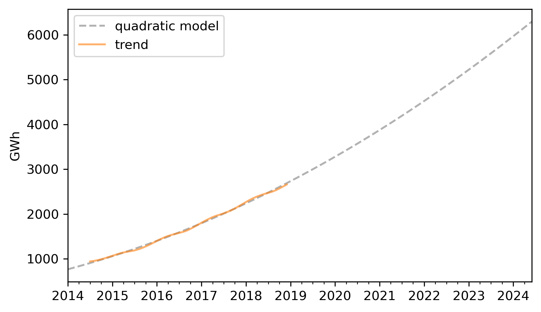
The quadratic model fits the past trend well. Now we can use the seasonal component to predict future seasonal variation.
monthly_averages = seasonal.groupby(seasonal.index.month).mean()
pred_seasonal = monthly_averages[pred_trend.index.month]
pred_seasonal.index = pred_trend.index
Finally, to compute retrodictions for past values and predictions for the future, we multiply the trend and the seasonal component.
pred = pred_trend * pred_seasonal
Here is the result along with the training data.
training.plot(label="training", **actual_options)
pred.plot(label="prediction", **pred_options)
decorate(ylabel="GWh")
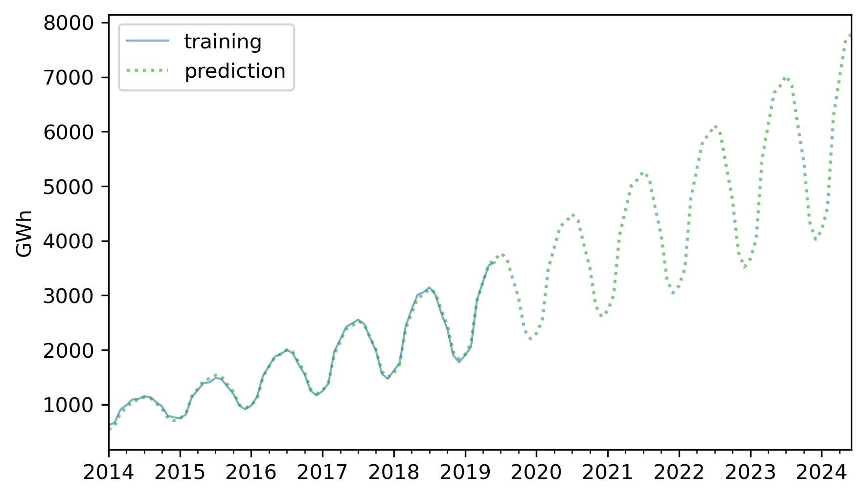
The retrodictions fit the training data well and the predictions seem plausible -- now let’s see if they turned out to be accurate. Here are the predictions along with the test data.
future = pred[test.index]
future.plot(label="prediction", **pred_options)
test.plot(label="actual", **actual_options)
decorate(ylabel="GWh")
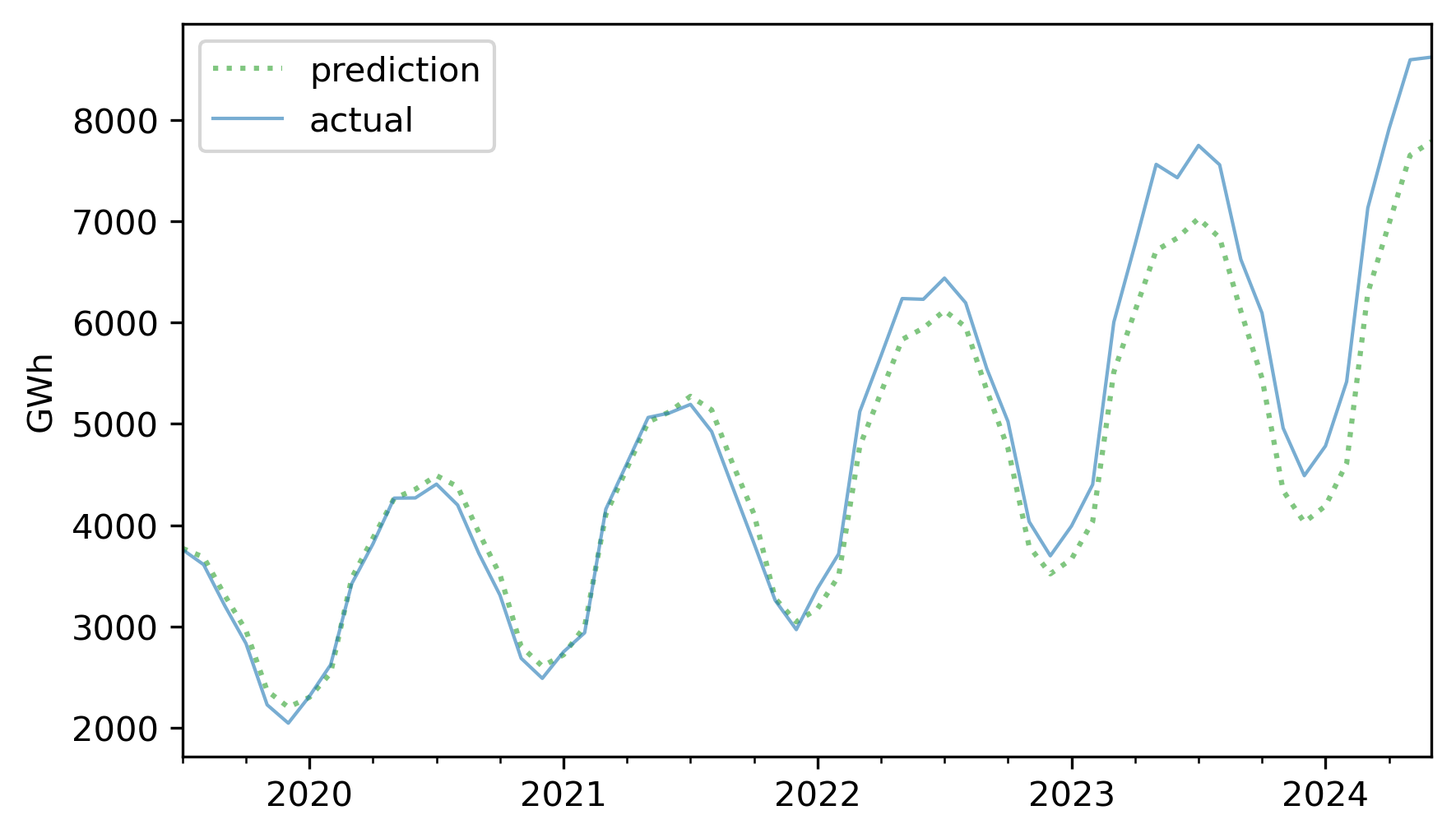
For the first three years, the predictions are very good. After that, it looks like actual growth exceeded expectations.
In this example, seasonal decomposition worked well for modeling and predicting solar production, but in the previous example, it was not very effective for nuclear production. In the next section, we’ll try a different approach, autoregression.

