Section 9.1 Flipping Coins
We’ll start with a simple example, based on an example in David MacKay’s book, Information Theory, Inference, and Learning Algorithms.
When Euro coins were introduced in 2002, a curious coin enthusiast spun a Belgian one-Euro coin on edge 250 times and noted that it landed with the heads side up 140 times and tails side up 110 times. If the coin is perfectly balanced, we expect only 125 heads, so this data suggests the coin is biased. On the other hand, we don’t expect to get exactly 125 heads every time, so it’s possible that the coin is actually fair, and the apparent deviation from the expected value is due to chance. To see whether that’s plausible, we can perform a hypothesis test.
We’ll use the following function to compute the absolute difference between the observed number and the expected number if the coin is fair.
n = 250
p = 0.5


def abs_deviation(heads):
    expected = n * p
    return np.abs(heads - expected)
In the observed data, this deviation is 15.
$ heads = 140
tails = 110

observed_stat = abs_deviation(heads)
observed_stat
np.float64(15.0)
If the coin is actually fair, we can simulate the coin-spinning experiment by generating a sequence of random strings -- either
'H' or 'T' with equal probability -- and counting the number of times 'H' appears.
def simulate_flips():
    flips = np.random.choice(["H", "T"], size=n)
    heads = np.sum(flips == "H")
    return heads
Each time we call this function, we get the outcome of a simulated experiment.
np.random.seed(1)
$ simulate_flips()
np.int64(119)
The following loop simulates the experiment many times, computes the deviation for each one, and uses a list comprehension to collect the results in a list.
simulated_stats = [abs_deviation(simulate_flips()) for i in range(10001)]
The result is a sample from the distribution of deviations under the assumption that the coin is fair. Here’s what the distribution of these values looks like.
from empiricaldist import Pmf

pmf_effects = Pmf.from_seq(simulated_stats)
pmf_effects.bar()

decorate(xlabel="Absolute deviation", ylabel="PMF")
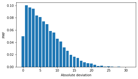
Values near 0 are the most common; values greater than 10 are less common. Remembering that the deviation in the observed data is 15, we see that deviations of that magnitude are rare, but not impossible. In this example, the simulated results equal or exceed 15 about 7.1% of the time.
$ (np.array(simulated_stats) >= 15).mean() * 100
np.float64(7.079292070792921)
So, if the coin is fair, we expect a deviation as big as the one we saw about 7.1% of the time, just by chance.
We can conclude that an effect of this size is not common, but it is certainly not impossible, even if the coin is fair. On the basis of this experiment, we can’t rule out the possibility that the coin is fair.
This example demonstrates the logic of statistical hypothesis testing.
-
We started with an observation, 140 heads out of 250 spins, and the hypothesis that the coin is biased -- that is, that the probability of heads differs from 50%.
-
We chose a test statistic that quantifies the size of the observed effect. In this example, the test statistic is the absolute deviation from the expected outcome.
-
We defined a null hypothesis, which is a model based on the assumption that the observed effect is due to chance. In this example, the null hypothesis is that the coin is fair.
-
Next, we computed a p-value, which is the probability of seeing the observed effect if the null hypothesis is true. In this example, the p-value is the probability of a deviation as big as 15 or bigger.
The last step is to interpret the result. If the p-value is small, we conclude that the effect would be unlikely to happen by chance. If it is large, we conclude that the effect could plausibly be explained by chance. And if it falls somewhere in the middle, as in this example, we can say that the effect is unlikely to happen by chance, but we can’t rule out the possibility.
All hypothesis tests are based on these elements -- a test statistic, a null hypothesis, and a p-value.

