Section 9.4 Testing a Correlation
We can use the same framework to test correlations. For example, in the NSFG data set, there is a correlation between birth weight and mother’s age -- older mothers have heavier babies, on average. But could this effect be due to chance?
To find out, we’ll start by preparing the data. From live births, we’ll select cases where the age of the mother and birth weight are known.
$ valid = live.dropna(subset=["agepreg", "totalwgt_lb"])
valid.shape
(9038, 244)
Then we’ll select the relevant columns.
ages = valid["agepreg"]
birthweights = valid["totalwgt_lb"]
The following function takes a tuple of
xs and ys and computes the magnitude of the correlation, positive or negative.
def abs_correlation(data):
    xs, ys = data
    corr = np.corrcoef(xs, ys)[0, 1]
    return np.abs(corr)
In the NSFG dataset, the correlation is about 0.07.
$ data = ages, birthweights
observed_corr = abs_correlation(data)
observed_corr
np.float64(0.0688339703541091)
The null hypothesis is that there is no correlation between mother’s age and birth weight. By shuffling the observed values, we can simulate a world where the distributions of age and birth weight are the same, but where the variables are unrelated.
The following function takes a tuple of
xs and ys, shuffles xs and returns a tuple containing the shuffled xs and the original ys. It would also work if we shuffled the ys instead, or shuffled both.
def permute(data):
    xs, ys = data
    new_xs = xs.values.copy()
    np.random.shuffle(new_xs)
    return new_xs, ys
The correlation of the shuffled values is usually close to 0.
$ abs_correlation(permute(data))
np.float64(0.0019269515502894465)
The following loop generates many shuffled datasets and computes the correlation of each one.
simulated_corrs = [abs_correlation(permute(data)) for i in range(1001)]
Here’s what the distribution of the results looks like. The vertical dotted line shows the observed correlation.
pmf = make_pmf(simulated_corrs, 0, 0.07)
pmf.plot()
plt.axvline(observed_corr, color="gray", ls=":")
decorate(xlabel="Absolute value of correlation", ylabel="Density")
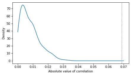
We can see that the observed correlation is in the tail of the distribution, with no visible area under the curve. If we try to compute a p-value, the result is 0, indicating that the correlation in the shuffled data did not exceed the observed value in any of the simulations.
$ compute_p_value(simulated_corrs, observed_corr)
np.float64(0.0)
Based on this calculation, we can conclude that the p-value is probably less that 1 per 1000, but it is not actually zero. It is unlikely for the correlation of the shuffled data to exceed the observed value -- but it is not impossible.
When the p-value is small, traditionally less than 0.05, we can say that the result is statistically significant. But this way of interpreting p-values has always been problematic, and it is slowly becoming less widely used.
One problem is that the traditional threshold is arbitrary and not appropriate for all applications. Another problem is that this use of "significant" is misleading because it suggests that the effect is important in practice. The correlation between mother’s age and birth weight is a good example -- it is statistically significant, but so small that it is not important.
An alternative is to interpret p-values qualitatively.
-
If a p-value is large, it is plausible that the observed effect could happen by chance.
-
If the p-value is small, we can often rule out the possibility that the effect is due to chance -- but we should remember that it could still be due to non-representative sampling or measurement errors.

