The Normal Distribution

Section 5.4 The Normal Distribution

Many things we measure in the real world follow a normal distribution, also known as a Gaussian distribution or a "bell curve". To see where these distributions come from, let’s consider a model of the way giant pumpkins grow. Suppose that each day, a pumpkin gains 1 pound if the weather is bad, 2 pounds if the weather is fair, and 3 pounds if the weather is good. And suppose the weather each day is bad, fair, or good with the same probability.

🔗

We can use the following function to simulate this model for n days and return the total of the weight gains. NumPy’s random module provides a choice function that generates an array of n random selections from a sequence of values.

🔗

Listing 5.4.1. Python Code

🔗

def simulate_growth(n):
    choices = [1, 2, 3]
    gains = np.random.choice(choices, n)
    return gains.sum()

Now suppose 1001 people grow giant pumpkins in different places with different weather. If we simulate the growth process for 100 days, we get a list of 1001 weights. The mean is close to 200 pounds and the standard deviation is about 8 pounds.

🔗

Listing 5.4.2. Python Code

🔗

$ sim_weights = [simulate_growth(100) for i in range(1001)]
m, s = np.mean(sim_weights), np.std(sim_weights)
m, s
(np.float64(199.37062937062936), np.float64(8.388630840376777))

To see whether the weights follow a normal distribution, we’ll use the following function, which takes a sample and makes a Cdf that represents a normal distribution with the same mean and standard deviation as the sample, evaluated over the range from 4 standard deviations below the mean to 4 standard deviations above.

🔗

Listing 5.4.3. Python Code

🔗

from scipy.stats import norm


def make_normal_model(data):
    m, s = np.mean(data), np.std(data)
    low, high = m - 4 * s, m + 4 * s
    qs = np.linspace(low, high, 201)
    ps = norm.cdf(qs, m, s)
    return Cdf(ps, qs, name="normal model")

Here’s how we use it

🔗

Listing 5.4.4. Python Code

🔗

cdf_model = make_normal_model(sim_weights)

Now we can make a Cdf that represents the distribution of the simulation results.

🔗

Listing 5.4.5. Python Code

🔗

cdf_sim_weights = Cdf.from_seq(sim_weights, name="simulation")

We’ll use the following function to compare the distributions. cdf_model and cdf_data are Cdf objects. xlabel is a string, and options is a dictionary of options that controls the way cdf_data is plotted.

🔗

Listing 5.4.6. Python Code

🔗

def two_cdf_plots(cdf_model, cdf_data, xlabel="", **options):
    cdf_model.plot(ls=":", color="gray")
    cdf_data.plot(**options)
    decorate(xlabel=xlabel, ylabel="CDF")

And here are the results comparing the normal model to the simulation.

🔗

Listing 5.4.7. Python Code

🔗

two_cdf_plots(cdf_model, cdf_sim_weights, xlabel="Weight (pounds)")

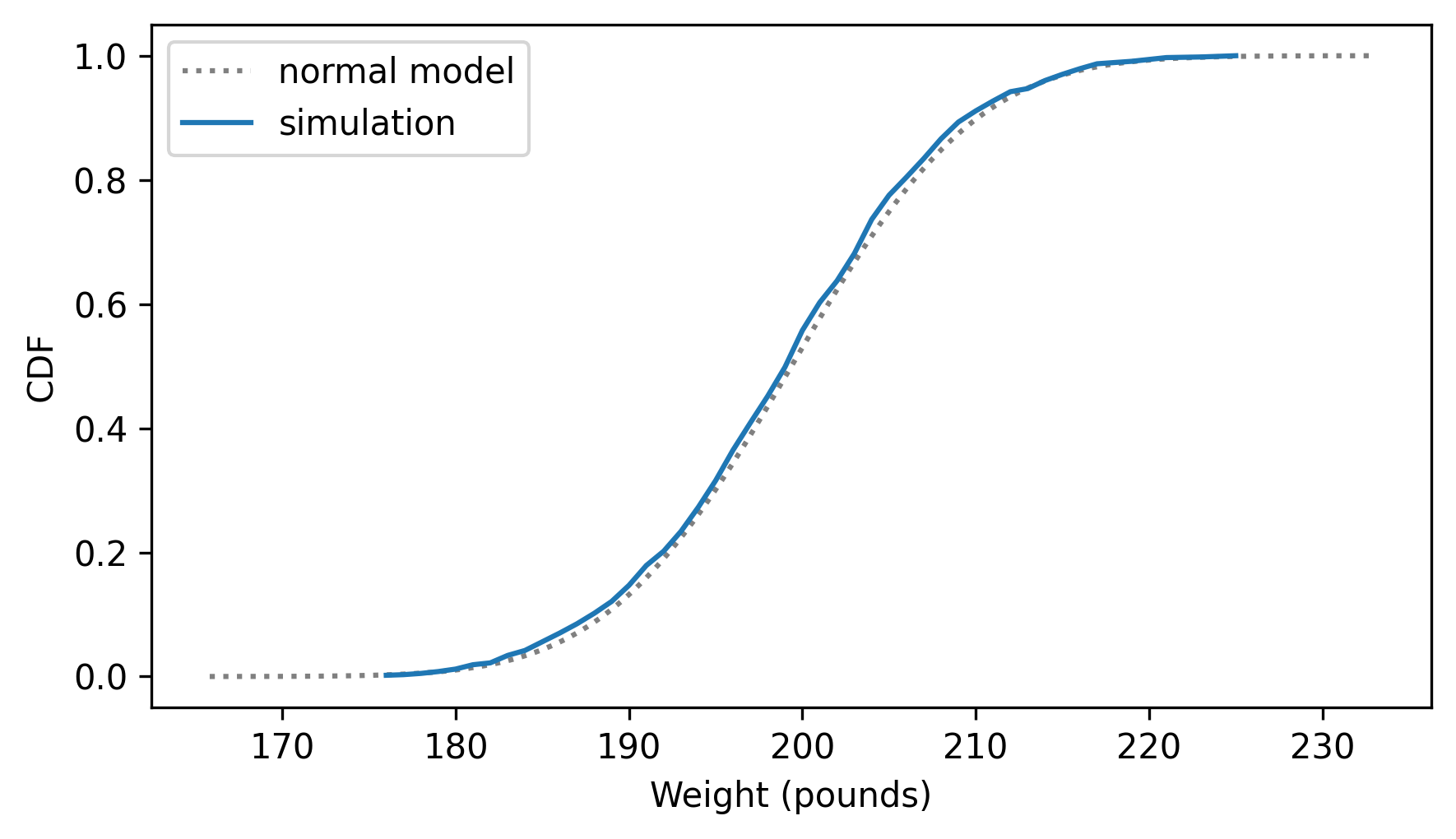
The normal model fits the distribution of the weights very well. In general, when we add up enough random factors, the sum tends to follow a normal distribution. That’s a consequence of the Central Limit Theorem, which we’ll come back to in Chapter 14.

🔗

But first let’s see how well the normal distribution fits real data. As an example, we’ll look at the distribution of birth weights in the National Survey of Family Growth (NSFG).

🔗

The following cells download the data files we need to read the data.

🔗

Listing 5.4.9. Python Code

🔗

download("https://github.com/AllenDowney/ThinkStats/raw/v3/nb/nsfg.py")
download("https://github.com/AllenDowney/ThinkStats/raw/v3/data/2002FemPreg.dct")
download("https://github.com/AllenDowney/ThinkStats/raw/v3/data/2002FemPreg.dat.gz")

Listing 5.4.10. Python Code

🔗

import nsfg

preg = nsfg.read_fem_preg()
birth_weights = preg["totalwgt_lb"].dropna()

The average of the birth weights is about 7.27 pounds, and the standard deviation is 1.4 pounds, but as we’ve seen, there are some outliers in this dataset that are probably errors.

🔗

Listing 5.4.11. Python Code

🔗

$ m, s = np.mean(birth_weights), np.std(birth_weights)
m, s
(np.float64(7.265628457623368), np.float64(1.40821553384062))

To reduce the effect of the outliers on the estimated mean and standard deviation, we’ll use the SciPy function trimboth to remove the highest and lowest values. With the trimmed data, the mean is a little lower and the standard deviation is substantially lower. We’ll use the trimmed data to make a normal model.

🔗

Listing 5.4.12. Python Code

🔗

$ from scipy.stats import trimboth

trimmed = trimboth(birth_weights, 0.01)
m, s = np.mean(trimmed), np.std(trimmed)
m, s
(np.float64(7.280883100022579), np.float64(1.2430657948614345))

With the trimmed data, the mean is a little lower and the standard deviation is substantially lower. We’ll use the trimmed data to make a normal model.

🔗

Listing 5.4.13. Python Code

🔗

cdf_model = make_normal_model(trimmed)

and compare it to the CDF of the data.

🔗

Listing 5.4.14. Python Code

🔗

cdf_birth_weight = Cdf.from_seq(birth_weights, name='data')

two_cdf_plots(cdf_model, cdf_birth_weight, xlabel="Birth weight (pounds)")

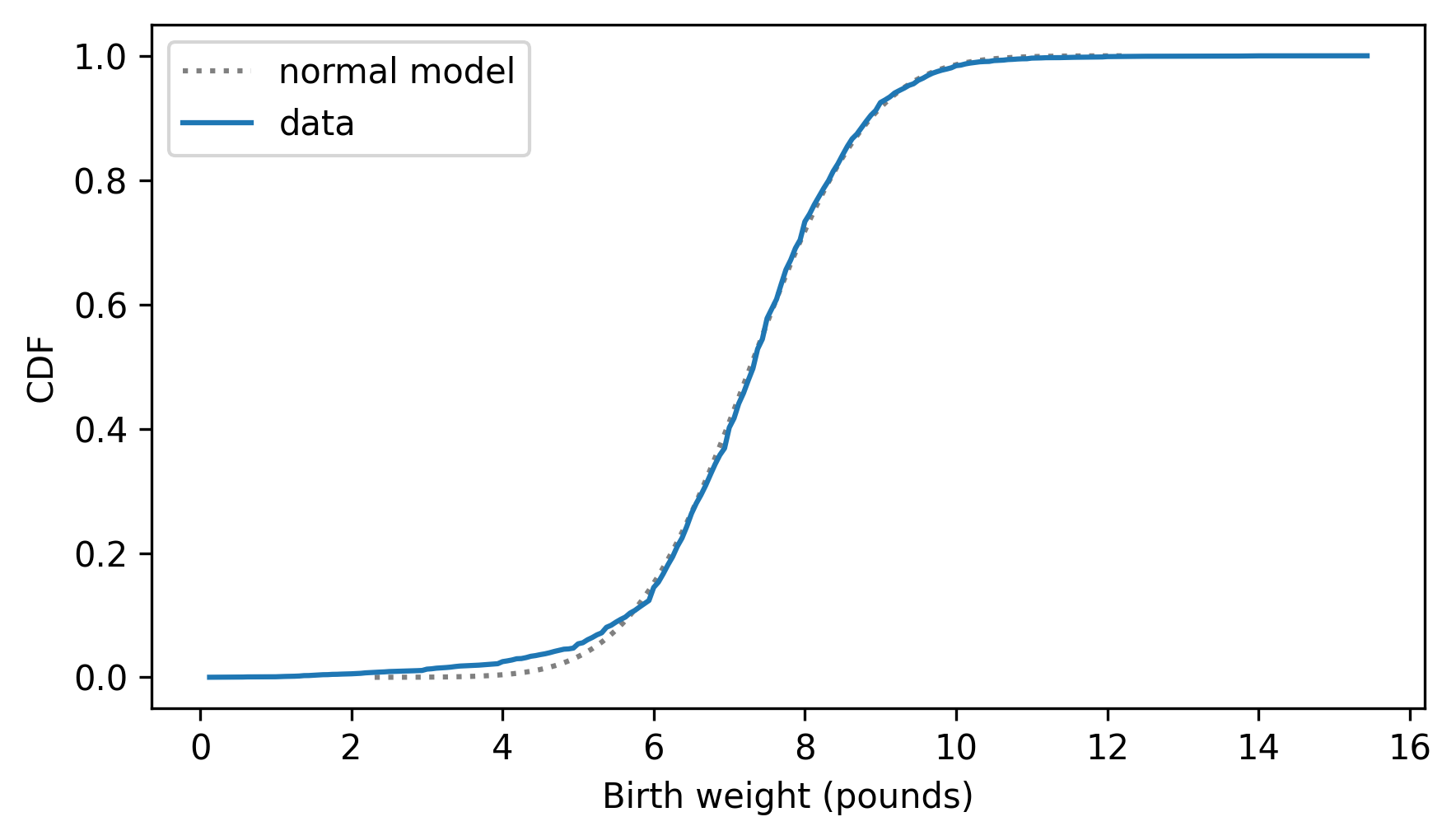
The normal model fits the data well except below 5 pounds, where the distribution of the data is to the left of the model — that is, the lightest babies are lighter than we’d expect in a normal distribution. The real world is usually more complicated than simple mathematical models.

🔗

Prev Top Next