Prediction

Section 12.3 Prediction

We can use the results from seasonal decomposition to predict the future. To demonstrate, we’ll use the following function to split the time series into a training series, which we’ll use to generate predictions, and a test series, which we’ll use to see whether they are accurate.

🔗

Listing 12.3.1. Python Code

🔗

def split_series(series, n=60):
    training = series.iloc[:-n]
    test = series.iloc[-n:]
    return training, test

With n=60, the duration of the test series is five years, starting in July 2019.

🔗

Listing 12.3.2. Python Code

🔗

$ training, test = split_series(nuclear)
test.index[0]
Timestamp('2019-07-31 00:00:00')

Now, suppose it’s June 2019 and you are asked to generate a five-year forecast for electricity production from nuclear generators. To answer this question, we’ll use the training data to make a model and then use the model to generate predictions. We’ll start with a seasonal decomposition of the training data.

🔗

Listing 12.3.3. Python Code

🔗

decomposition = seasonal_decompose(training, model="additive", period=12)
trend = decomposition.trend

Now we’ll fit a linear model to the trend. The explanatory variable, months, is the number of months from the beginning of the series.

🔗

Listing 12.3.4. Python Code

🔗

import statsmodels.formula.api as smf

months = np.arange(len(trend))
data = pd.DataFrame({"trend": trend, "months": months}).dropna()
results = smf.ols("trend ~ months", data=data).fit()

Here is a summary of the results.

🔗

Listing 12.3.5. Python Code

🔗

from thinkstats import display_summary

display_summary(results)

Table 12.3.6.

🔗

	coef	std err	t	P>\|t\|	[0.025	0.975]
Intercept	6.482e+04	131.524	492.869	0.000	6.46e+04	6.51e+04
months	10.9886	1.044	10.530	0.000	8.931	13.046

Table 12.3.7.

🔗

R-squared:

0.3477

The \(R^2\) value is about 0.35, which suggests that the model does not fit the data particularly well. We can get a better sense of that by plotting the fitted line. We’ll use the predict method to compute expected values for the training and test data.

🔗

Listing 12.3.8. Python Code

🔗

months = np.arange(len(training) + len(test))
df = pd.DataFrame({"months": months})
pred_trend = results.predict(df)
pred_trend.index = nuclear.index

Here’s the trend component and the linear model.

🔗

Listing 12.3.9. Python Code

🔗

trend.plot(**trend_options)
pred_trend.plot(label="linear model", **model_options)
decorate(ylabel="GWh")

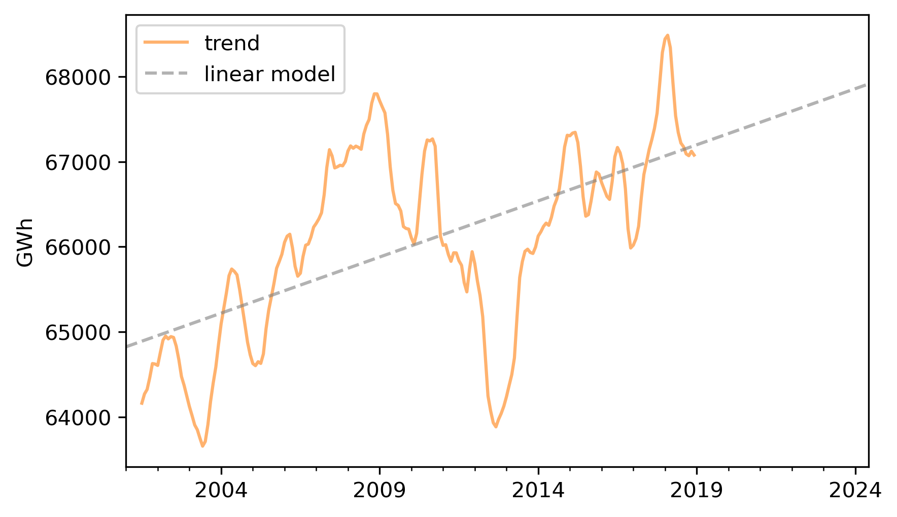
There’s a lot going on that’s not captured by the linear model, but it looks like there is a generally increasing trend.

🔗

Next we’ll use the seasonal component from the decomposition to compute a Series of monthly averages.

🔗

Listing 12.3.11. Python Code

🔗

seasonal = decomposition.seasonal
monthly_averages = seasonal.groupby(seasonal.index.month).mean()

We can predict the seasonal component by looking up the dates from the fitted line in monthly_averages.

🔗

Listing 12.3.12. Python Code

🔗

pred_seasonal = monthly_averages[pred_trend.index.month]
pred_seasonal.index = pred_trend.index

Finally, to generate predictions, we’ll add the seasonal component to the trend.

🔗

Listing 12.3.13. Python Code

🔗

pred = pred_trend + pred_seasonal

Here’s the training data and the predictions.

🔗

Listing 12.3.14. Python Code

🔗

pred.plot(label="prediction", **pred_options)
training.plot(label="training", **actual_options)
decorate(ylabel="GWh")

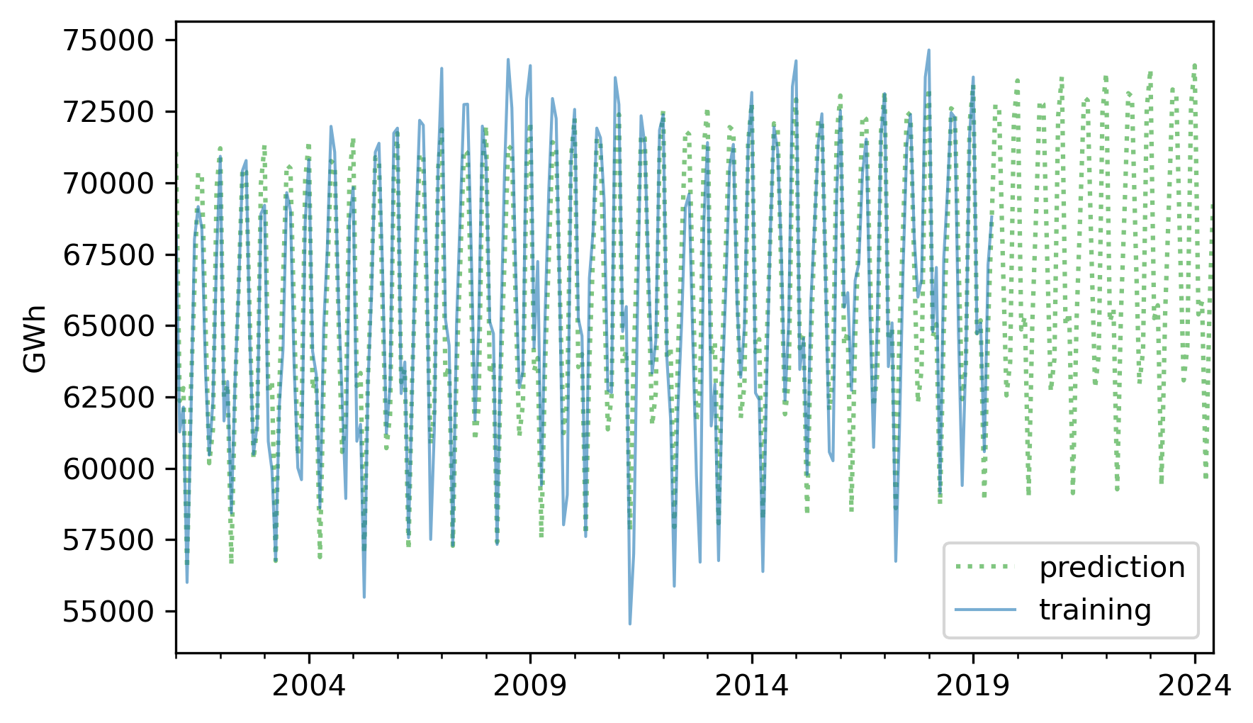
The predictions fit the training data reasonably well, and the forecast looks like a reasonable projection, based on the assumption that the long-term trend will continue.

🔗

Now, from the vantage point of the future, let’s see how accurate this forecast turned out to be. Here are the predicted and actual values for the five-year interval from July 2019.

🔗

Listing 12.3.16. Python Code

🔗

forecast = pred[test.index]
forecast.plot(label="predicted", **pred_options)
test.plot(label="actual", **actual_options)
decorate(ylabel="GWh")

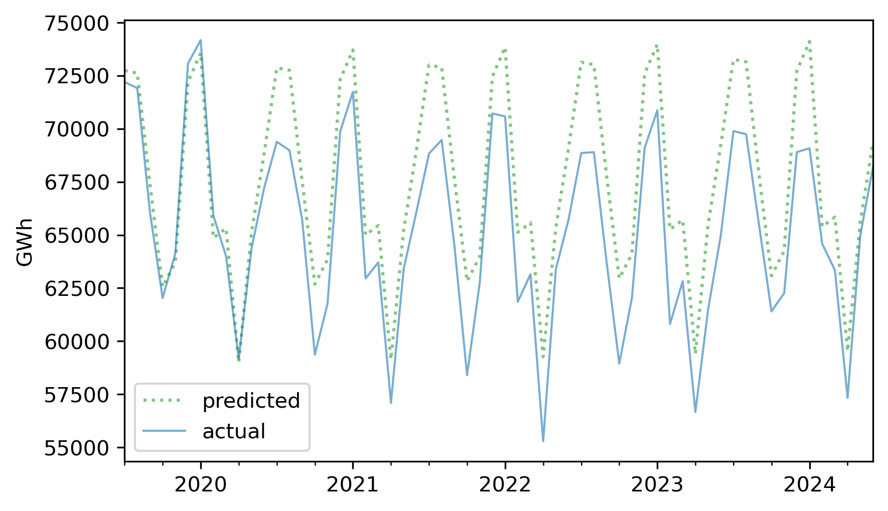
The first year of the forecast was pretty good, but production from nuclear reactors in 2020 was lower than expected -- possibly due to the COVID-19 pandemic -- and it never returned to the long-term trend.

🔗

To quantify the accuracy of the predictions, we’ll use the mean absolute percentage error (MAPE), which the following function computes.

🔗

Listing 12.3.18. Python Code

🔗

def MAPE(predicted, actual):
    ape = np.abs(predicted - actual) / actual
    return np.mean(ape) * 100

In this example, the predictions are off by 3.81% on average.

🔗

Listing 12.3.19. Python Code

🔗

$ MAPE(forecast, test)
np.float64(3.811940747879257)

We’ll come back to this example later in the chapter and see if we can do better with a different model.

🔗

Prev Top Next