Section 6.1 Comparing Distributions
In the previous chapter, when we compared discrete distributions, we used a bar plot to show their probability mass functions (PMFs). When we compared continuous distributions, we used a line plot to show their cumulative distribution functions (CDFs).
For the discrete distributions, we could also have used CDFs. For example, here’s the PMF of a Poisson distribution with
lam=2.2, which is a good model for the distribution of household size in the NSFG data.
The following cells download the data files and install
statadict, which we need to read the data.
download("https://github.com/AllenDowney/ThinkStats/raw/v3/nb/nsfg.py")
download("https://github.com/AllenDowney/ThinkStats/raw/v3/data/2002FemResp.dct")
download("https://github.com/AllenDowney/ThinkStats/raw/v3/data/2002FemResp.dat.gz")
try:
    import statadict
except ImportError:
    %pip install statadict
We can use
read_fem_resp to read the respondent data file.
from nsfg import read_fem_resp

resp = read_fem_resp()
Next we’ll select household sizes for people 25 and older.
older = resp.query("age >= 25")
num_family = older["numfmhh"]
And make a
Pmf that represents the distribution of responses.
from empiricaldist import Pmf

pmf_family = Pmf.from_seq(num_family, name="data")
Here’s another
Pmf that represents a Poisson distribution with the same mean.
from thinkstats import poisson_pmf

lam = 2.2
ks = np.arange(11)
ps = poisson_pmf(ks, lam)

pmf_poisson = Pmf(ps, ks, name="Poisson model")
And here’s how the distribution of the data compares to the Poisson model.
from thinkstats import two_bar_plots

two_bar_plots(pmf_family, pmf_poisson)
decorate(xlabel="Number of family members")
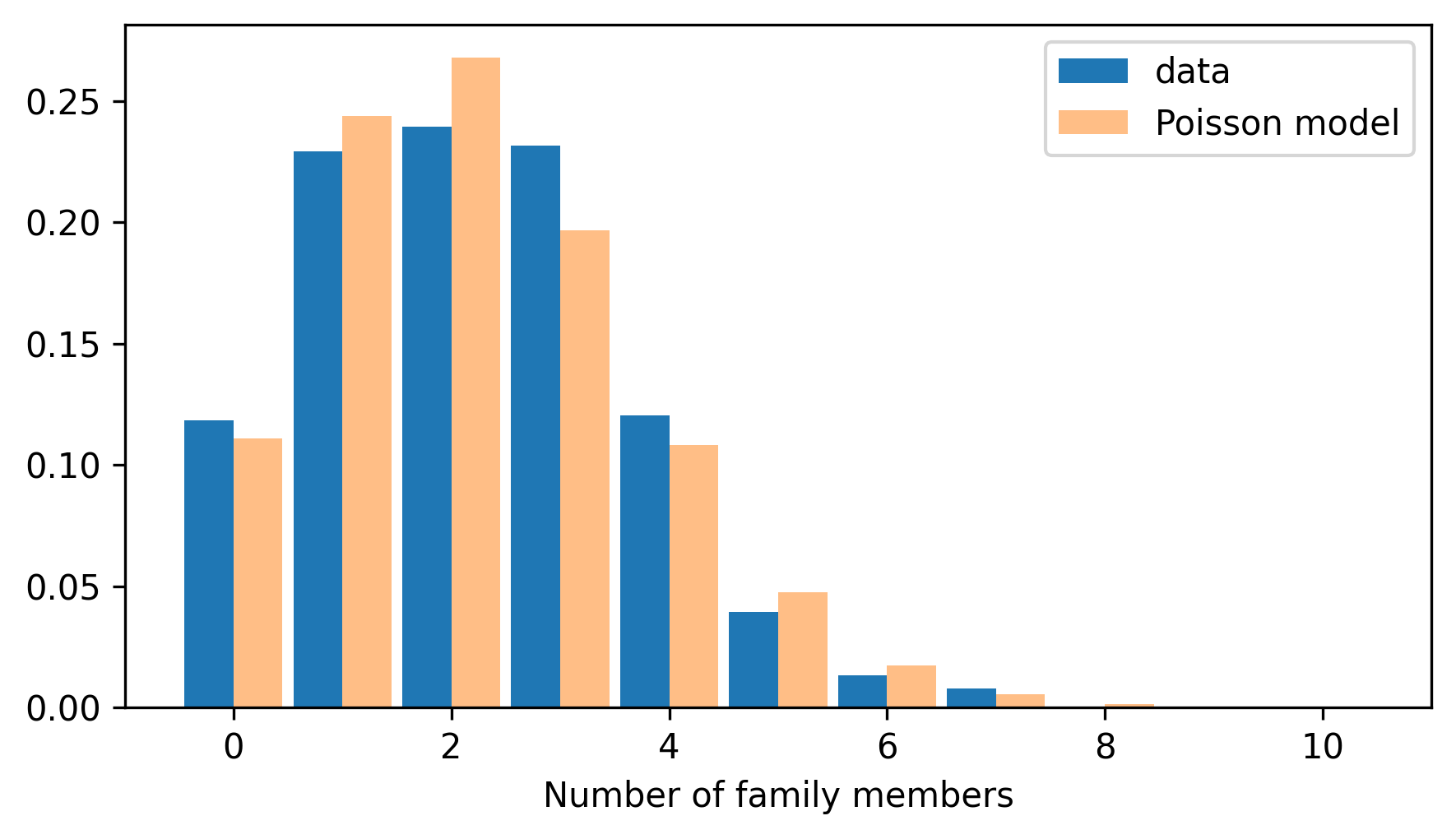
Comparing the PMFs, we can see that the model fits the data well, but with some deviations.
To get a sense of how substantial those deviations are, it can be helpful to compare CDFs. We can use
make_cdf to compute the CDFs of the data and the model.
cdf_family = pmf_family.make_cdf()
cdf_poisson = pmf_poisson.make_cdf()
Here’s what they look like.
from thinkstats import two_cdf_plots

two_cdf_plots(cdf_poisson, cdf_family)
decorate(xlabel="Number of family members")
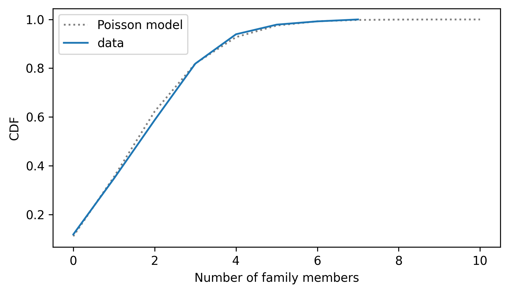
When we compare CDFs, the deviations are less prominent, but we can see where and how the distributions differ. PMFs tend to emphasize small differences — sometimes CDFs provide a better sense of the big picture.
CDFs also work well with continuous data. As an example, let’s look at the distribution of birth weights again, which is in the NSFG pregnancy file.
download("https://github.com/AllenDowney/ThinkStats/raw/v3/data/2002FemPreg.dct")
download("https://github.com/AllenDowney/ThinkStats/raw/v3/data/2002FemPreg.dat.gz")
from nsfg import read_fem_preg

preg = read_fem_preg()
birth_weights = preg["totalwgt_lb"].dropna()
Here is the code we used in the previous chapter to fit a normal model to the data.
from scipy.stats import trimboth
from thinkstats import make_normal_model

trimmed = trimboth(birth_weights, 0.01)
cdf_model = make_normal_model(trimmed)
And here’s the distribution of the data compared to the normal model.
from empiricaldist import Cdf

cdf_birth_weight = Cdf.from_seq(birth_weights, name="sample")
two_cdf_plots(cdf_model, cdf_birth_weight, xlabel="Birth weight (pounds)")
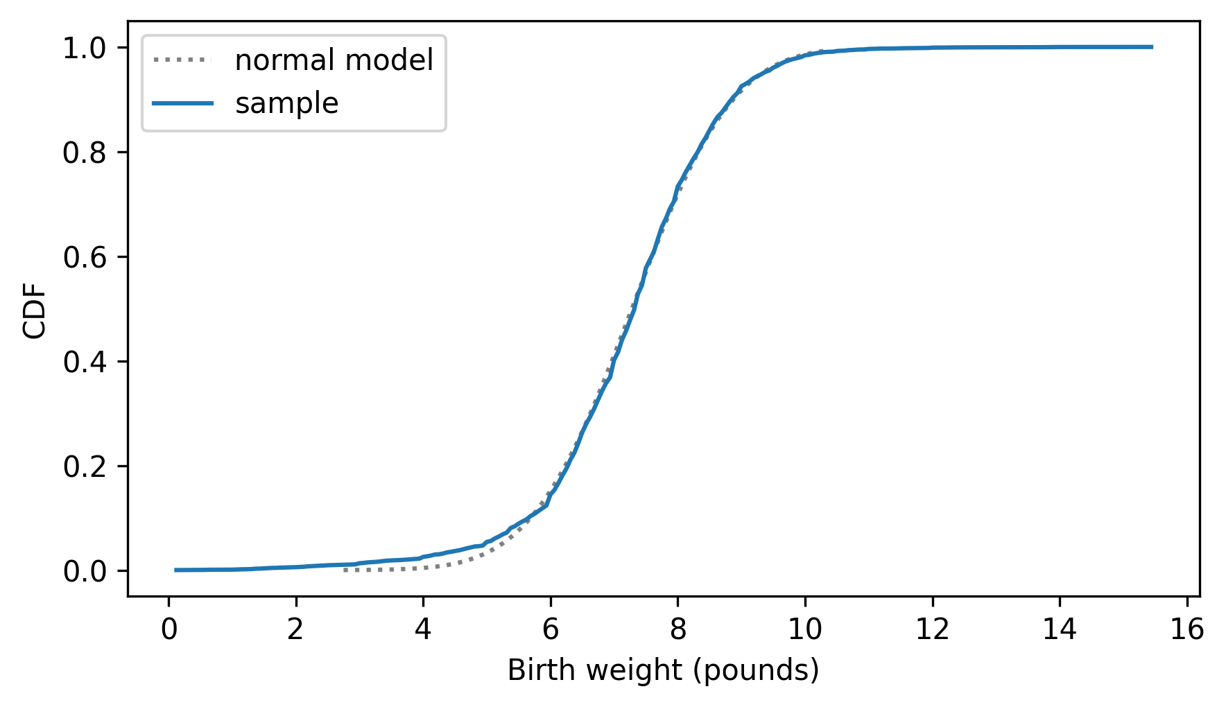
As we saw in the previous chapter, the normal model fits the data well except in the range of the lightest babies.
In my opinion, CDFs are usually the best way to compare data to a model. But for audiences that are not familiar with CDFs, there is one more option: probability density functions.

