Testing Proportions

Section 9.5 Testing Proportions

As a final example, let’s consider a case where the choice of the test statistic takes some thought. Suppose you run a casino and you suspect that a customer is using a crooked die -- that is, one that has been modified to make one of the faces more likely than the others. You apprehend the alleged cheater and confiscate the die, but now you have to prove that it is crooked. You roll the die 60 times and record the frequency of each outcome from 1 to 6. Here are the results in a Hist object.

🔗

Listing 9.5.1. Python Code

🔗

$ from empiricaldist import Hist

qs = np.arange(1, 7)
freqs = [8, 9, 19, 5, 8, 11]
observed = Hist(freqs, qs)
observed.index.name = "outcome"
observed
outcome
1     8
2     9
3    19
4     5
5     8
6    11
dtype: int64

On average you expect each value to appear 10 times. In this dataset, the value 3 appears more often than expected, and the value 4 appears less often. But could these differences happen by chance?

🔗

To test this hypothesis, we’ll start by computing the expected frequency for each outcome.

🔗

Listing 9.5.2. Python Code

🔗

num_rolls = observed.sum()
outcomes = observed.qs
expected = Hist(num_rolls / 6, outcomes)

The following function takes the observed and expected frequencies and computes the sum of the absolute differences.

🔗

Listing 9.5.3. Python Code

🔗

def total_abs_deviation(observed):
    return np.sum(np.abs(observed - expected))

In the observed dataset, this test statistic is 20.

🔗

Listing 9.5.4. Python Code

🔗

$ observed_dev = total_abs_deviation(observed)
observed_dev
np.float64(20.0)

The following function takes the observed data, simulates rolling a fair die the same number of times, and returns a Hist object that contains the simulated frequencies.

🔗

Listing 9.5.5. Python Code

🔗

def simulate_dice(observed):
    num_rolls = np.sum(observed)
    rolls = np.random.choice(observed.qs, num_rolls, replace=True)
    hist = Hist.from_seq(rolls)
    return hist

The following loop simulates the experiment many times and computes the total absolute deviation for each one.

🔗

Listing 9.5.6. Python Code

🔗

simulated_devs = [total_abs_deviation(simulate_dice(observed)) for i in range(1001)]

Here’s what the distribution of the test statistic looks like under the null hypothesis. Notice that the total is always even, because every time an outcome appears more often than expected, another outcome has to appear less often.

🔗

Listing 9.5.7. Python Code

🔗

pmf_devs = Pmf.from_seq(simulated_devs)
pmf_devs.bar()

decorate(xlabel="Total absolute deviation", ylabel="PMF")

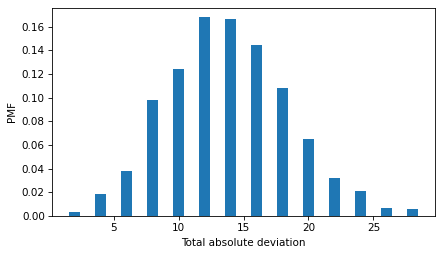
We can see that a total deviation of 20 is not unusual -- the p-value is about 13%, which means that we can’t be sure the die is crooked.

🔗

Listing 9.5.9. Python Code

🔗

$ compute_p_value(simulated_devs, observed_dev)
np.float64(0.13086913086913088)

But the test statistic we chose was not the only option. For a problem like this, it would be more conventional to use the chi-squared statistic, which we can compute like this.

🔗

Listing 9.5.10. Python Code

🔗

def chi_squared_stat(observed):
    diffs = (observed - expected) ** 2
    return np.sum(diffs / expected)

Squaring the deviations (rather than taking absolute values) gives more weight to large deviations. Dividing through by expected standardizes the deviations -- although in this case it has no effect on the results because the expected frequencies are all equal.

🔗

Listing 9.5.11. Python Code

🔗

$ observed_chi2 = chi_squared_stat(observed)
observed_chi2
np.float64(11.6)

The chi-squared statistic of the observed data is 11.6. By itself, this number doesn’t mean very much, but we can compare it to the results from the simulated rolls. The following loop generates many simulated datasets and computes the chi-squared statistic for each one.

🔗

Listing 9.5.12. Python Code

🔗

simulated_chi2 = [chi_squared_stat(simulate_dice(observed)) for i in range(1001)]

Here’s what the distribution of this test statistic looks like under the null hypothesis. The shaded region shows the results that exceed the observed value.

🔗

Listing 9.5.13. Python Code

🔗

pmf = make_pmf(simulated_chi2, 0, 20)
pmf.plot()
fill_tail(pmf, observed_chi2, "right")
decorate(xlabel="Chi-Squared statistic", ylabel="Density")

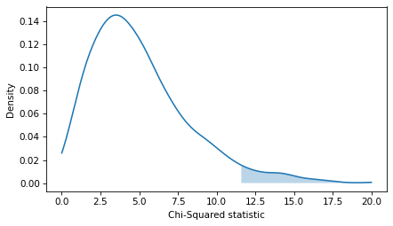
Again, the area of the shaded region is the p-value.

🔗

Listing 9.5.15. Python Code

🔗

$ compute_p_value(simulated_chi2, observed_chi2)
np.float64(0.04495504495504495)

The p-value using the chi-squared statistic is about 0.04, substantially smaller than what we got using total deviation, 0.13. If we take the 5% threshold seriously, we would consider this effect statistically significant. But considering the two tests together, I would say that the results are inconclusive. I would not rule out the possibility that the die is crooked, but I would not convict the accused cheater.

🔗

This example demonstrates an important point: the p-value depends on the choice of test statistic and the model of the null hypothesis, and sometimes these choices determine whether an effect is statistically significant or not.

🔗

Prev Top Next