The Poisson Distribution

Section 5.2 The Poisson Distribution

As another example where the outcomes of sports events follow predictable patterns, let’s look at the number of goals scored in ice hockey games.

🔗

We’ll start by simulating a 60-minute game, which is 3600 seconds, assuming that the teams score a total of 6 goals per game, on average, and that the goal-scoring probability, p, is the same during any second.

🔗

Listing 5.2.1. Python Code

🔗

$ n = 3600
m = 6
p = m / 3600
p
0.0016666666666666668

Now we can use the following function to simulate n seconds and return the total number of goals scored.

🔗

Listing 5.2.2. Python Code

🔗

def simulate_goals(n, p):
    return flip(n, p).sum()

If we simulate many games, we can confirm that the average number of goals per game is close to 6.

🔗

Listing 5.2.3. Python Code

🔗

$ goals = [simulate_goals(n, p) for i in range(1001)]
np.mean(goals)
np.float64(6.021978021978022)

We could use the binomial distribution to model these results, but when n is large and p is small, the results are also well-modeled by a Poisson distribution, which is specified by a value usually denoted with the Greek letter λ (lambda), represented in code with the variable lam. lam represents the goal-scoring rate, which is 6 goals per game in the example.

🔗

The PMF of the Poisson distribution is easy to compute — given lam, we can use the following function to compute the probability of seeing k goals in a game.

🔗

Listing 5.2.4. Python Code

🔗

from scipy.special import factorial


def poisson_pmf(k, lam):
    """Compute the Poisson PMF.

    k (int or array-like): The number of occurrences
    lam (float): The rate parameter (λ) of the Poisson distribution

    returns: float or ndarray
    """
    return (lam**k) * np.exp(-lam) / factorial(k)

SciPy provides the factorial function, which computes the product of the integers from 1 to k.

🔗

If we call poisson_pmf with a range of k values, we can make a Pmf that represents the distribution of outcomes, and confirm that the mean of the distribution is close to 6.

🔗

Listing 5.2.5. Python Code

🔗

lam = 6
ks = np.arange(20)
ps = poisson_pmf(ks, lam)
pmf_poisson = Pmf(ps, ks, name="Poisson model")

Listing 5.2.6. Python Code

🔗

$ pmf_poisson.normalize()
pmf_poisson.mean()
np.float64(5.999925498375129)

The following figure compares the results from the simulation to the Poisson distribution with the same mean.

🔗

Listing 5.2.7. Python Code

🔗

pmf_sim = Pmf.from_seq(goals, name="simulation")

two_bar_plots(pmf_sim, pmf_poisson)
decorate(xlabel="Goals", ylabel="PMF")

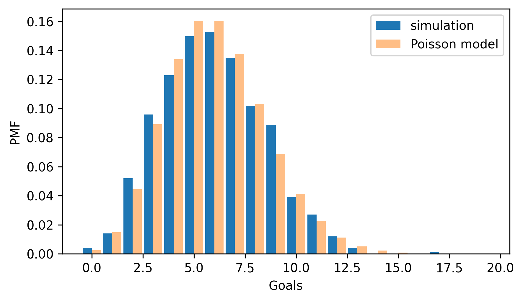
The distributions are similar except for small differences due to random variation. That should not be surprising, because the simulation and the Poisson model are based on the same assumption that the probability of scoring a goal is the same during any second of the game. So a stronger test is to see how well the model fits real data.

🔗

I downloaded results of every game of the National Hockey League (NHL) 2023-2024 regular season. I extracted information about goals scored during 60 minutes of regulation play, not including overtime or tie-breaking shootouts. The results are in an HDF file with one key for each game, and a list of times, in seconds since the beginning of the game, when a goal was scored.

🔗

Raw data downloaded from https://www.hockey-reference.com/leagues/NHL_2024_games.html on July 16, 2024.

🔗

Listing 5.2.9. Python Code

🔗

download("https://github.com/AllenDowney/ThinkStats/raw/v3/data/nhl_2023_2024.hdf")

Here’s how we read the keys from the file.

🔗

Listing 5.2.10. Python Code

🔗

$ filename = "nhl_2023_2024.hdf"

with pd.HDFStore(filename, "r") as store:
    keys = store.keys()

len(keys), keys[0]
(1312, '/202310100PIT')

There were 1312 games during the regular season. Each key contains the date of the game and a three-letter abbreviation for the home team. We can use read_hdf to look up a key and get the list of times when a goal was scored.

🔗

Listing 5.2.11. Python Code

🔗

$ times = pd.read_hdf(filename, key=keys[0])
times
0     424
1    1916
2    2137
3    3005
4    3329
5    3513
dtype: int64

In the first game of the season, six goals were scored, the first after 424 seconds of play, the last after 3513 seconds — with only 87 seconds left in the game.

🔗

Listing 5.2.12. Python Code

🔗

$ 3600 - times[5]
np.int64(87)

The following loop reads the results for all games, counts the number of goals in each one, and stores the results in a list.

🔗

Listing 5.2.13. Python Code

🔗

goals = []

for key in keys:
    times = pd.read_hdf(filename, key=key)
    n = len(times)
    goals.append(n)

The average number of goals per game is just over 6.

🔗

Listing 5.2.14. Python Code

🔗

$ lam = np.mean(goals)
lam
np.float64(6.0182926829268295)

We can use poisson_pmf to make a Pmf that represents a Poisson distribution with the same mean as the data, and compare that to the Pmf of the data.

🔗

Listing 5.2.15. Python Code

🔗

ps = poisson_pmf(ks, lam)
pmf_poisson = Pmf(ps, ks, name="Poisson model")

Listing 5.2.16. Python Code

🔗

pmf_goals = Pmf.from_seq(goals, name="goals scored")

two_bar_plots(pmf_goals, pmf_poisson)
decorate(xlabel="Goals", ylabel="PMF")

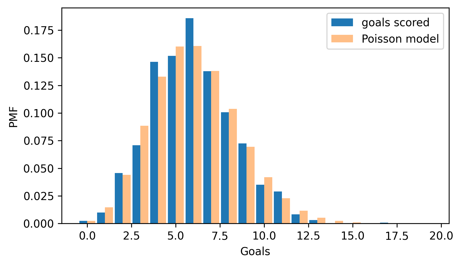
The Poisson distribution fits the data well, which suggests that it is a good model of the goal-scoring process in hockey.

🔗

Prev Top Next